Business Problem:
Picture this: You're organizing a company retreat, a school assembly, or perhaps a community gathering. As the organizer, you're keen to ensure everyone is engaged and enjoying themselves. But how can you gauge the collective mood of the group? That's where this project comes in. The aim is to develop a system capable of analyzing group images to identify the emotions of the individuals within them. By employing deep learning models and algorithms, we aim to identify whether the group is demonstrating happiness, enthusiasm, apprehension, or any other emotional state.
Such a system holds immense potential for various applications. For businesses, it could provide valuable insights into employee satisfaction during team-building events or meetings. In educational settings, it could help educators assess student engagement during lectures or group activities. Even event organizers could leverage this tool to ensure attendees are having a positive experience. Ultimately, by decoding group emotions through visual data, we strive to enhance social dynamics and foster environments favorable to collective well-being and productivity. 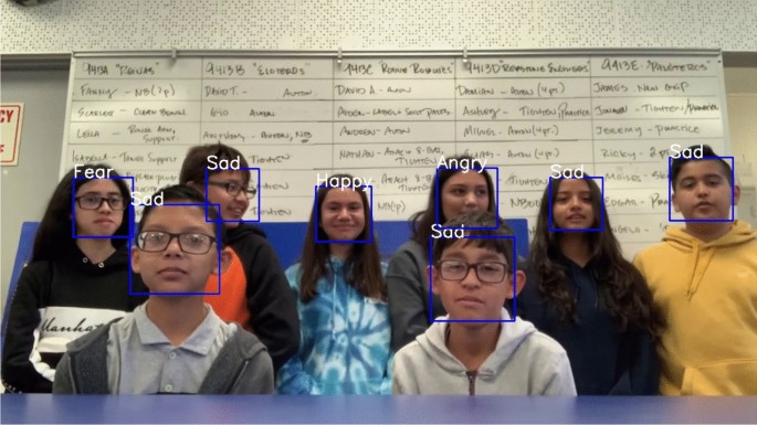
Existing Solution and Limitations:
Understanding group emotions from group images is challenging because it involves identifying how each person in the group feels, which can be different for everyone. Traditional methods often treat the whole group as feeling the same way, missing the individual emotions. Also, analyzing group pictures accurately means needing to pick out emotions from both the whole group and each person's face, which can be hard because of different lighting and facial expressions. Plus, emotions can be subtle and vary based on the situation, making it tricky to get it right. Finally, doing this quickly and accurately is important for tasks like managing events or customer interactions.
Proposed Solution:
This project aims to redefine the way we perceive and interpret group emotions by implementing an approach that takes into account the individual emotions within a group. Instead of solely analyzing group images as a whole, our solution involves employing deep learning models to extract emotions of individuals given group images. We strive to create a comprehensive understanding of group emotions that captures the rich diversity of feelings present among group members.
Technical Objectives
- Face Detection and Extraction:
- Given an image of a group of people, extract and isolate faces of individual people in the image.
- Use pretrained models such as YOLOv8, YOLOv8 Face, Single-Shot Multibox Detector (SSD), or non-ML algorithmic techniques such as HaarCascade to extract these individual faces.
- Emotion Classification:
- Once the individual faces have been extracted, identify the emotion of each of the faces in the given image. Use techniques such as majority voting to identify the emotion of the entire group.
- Use Facial Attribute Analysis from DeepFace library to analyze individual emotions. Feel free to explore other Facial Emotion Recognition models. Labeling, Validation and Evaluation
- To enable performance validation of the pipeline, we have scrapped about 3000 group images from the internet.
- Label all or a subset of images manually for faces and emotions of each of the faces. You can use a tool such as Label Studio for the same. If you choose to label a subset of images, ensure that there is a diversity in the kind of images you include in your subset.
- Use the labeled images to validate the performance of your solution. Benchmark your solution for latency, as well as against statistical metrics such as Intersection of Union (IoU), Accuracy, Precision, Recall etc.
DeepFace library comes with support for both - face detection/extraction and Emotion Recognition. However, since it comes with a plethora of models and options (called backends), you need to weigh in the tradeoff between statistical performance and scalability. Explore as many options as you can to ensure that your analysis and solution are comprehensive. Also, consider exploring Super Resolution techniques for improving image quality.
!gcloud config list --format "text(core.project)"
!gcloud auth list
FILE_ID = "17UoqIa5vzUVglQccnSDtA3w6ZYggrHRh"
ZIP_PATH = "/content/group_emotion_dataset.zip"
EXTRACT_DIR = "/content/group_emotion_dataset"
GCS_BUCKET = "ranjana-group-emotion-data" # <-- change this
GCS_PREFIX = "group_emotion_data" # <-- change if you want
!gsutil ls gs://{GCS_BUCKET} >/dev/null && echo "Bucket access OK" || echo "No access to bucket"
!pip -q install gdown
import gdown
url = f"https://drive.google.com/uc?id={FILE_ID}"
gdown.download(url, ZIP_PATH, quiet=False)
import os
print("ZIP exists:", os.path.exists(ZIP_PATH))
print("ZIP size:", os.path.getsize(ZIP_PATH))
import zipfile, os
os.makedirs(EXTRACT_DIR, exist_ok=True)
with zipfile.ZipFile(ZIP_PATH, "r") as z:
z.extractall(EXTRACT_DIR)
# quick peek
for root, dirs, files in os.walk(EXTRACT_DIR):
print("Top extracted folder:", root)
print("Top extracted directory:", dirs)
print("Example files:", files[:5])
SRC_DIR = os.path.join(EXTRACT_DIR, "Scraped-Dataset for GroupEmotion")
assert os.path.exists(SRC_DIR), f"Not found: {SRC_DIR}"
print("Source folder:", SRC_DIR)
print("Example entries:", os.listdir(SRC_DIR)[:10])
!gsutil -m rsync -r "{SRC_DIR}" "gs://{GCS_BUCKET}/{GCS_PREFIX}"
Exploratory Data Analysis
import random
from google.cloud import storage
client = storage.Client()
bucket = client.bucket(GCS_BUCKET)
# Collect image blobs (no stdout flooding)
image_blobs = [
blob for blob in client.list_blobs(bucket, prefix=GCS_PREFIX)
if blob.name.lower().endswith((".jpg", ".jpeg", ".png", ".webp"))
]
print("Image count:", len(image_blobs))
assert len(image_blobs) > 0, "No images found in the given GCS path."
import os
# Pick one at random
blob = random.choice(image_blobs)
print("Selected image:", blob.name)
LOCAL_PATH = "/content/random_image.jpg"
blob.download_to_filename(LOCAL_PATH)
print("Downloaded to:", LOCAL_PATH)
from PIL import Image
from IPython.display import display
display(Image.open(LOCAL_PATH))

assert len(image_blobs) >= 2, "Need at least 2 images in this prefix."
picked = random.sample(image_blobs, 2)
local_paths = []
os.makedirs("/content/bakeoff", exist_ok=True)
for i, b in enumerate(picked, 1):
lp = f"/content/bakeoff/img{i}_" + os.path.basename(b.name)
b.download_to_filename(lp)
local_paths.append(lp)
print(f"Downloaded {i}:", b.name, "->", lp)
local_paths
display(Image.open(local_paths[0]))

display(Image.open(local_paths[1]))

Expected Task-flow
- Detect faces from group images
- Extract faces.
- Analyze Emotions.
- Calculate avg emotions.
Step-1:Detect Faces
Compare DeepFace/RetinaFace with YOLO11 for face detection
!pip -q install --upgrade "protobuf>=6.31.1,<7"
!pip -q install --upgrade "numpy==1.26.4" "pillow==11.1.0"
!pip -q install --upgrade opencv-python-headless
!pip -q install --upgrade deepface ultralytics
# Keep platform-compatible core libraries
!pip install -q protobuf==4.25.3
!pip install -q --upgrade numpy pillow
# Install only what you need
!pip install -q opencv-python-headless
!pip install -q deepface
!pip install -q ultralytics
import numpy
import protobuf
import cv2
from deepface import DeepFace
from ultralytics import YOLO
print("NumPy:", numpy.__version__)
print("Protobuf:", protobuf.__version__)
print("OpenCV:", cv2.__version__)
! pip install protobuf
import sys
import os
# Uninstall all potentially conflicting packages first
# This helps in starting with a cleaner slate for dependency resolution
!pip uninstall -y fer deepface ultralytics opencv-python opencv-python-headless numpy protobuf Pillow
# Install a protobuf version known to be more compatible with TensorFlow/Ultralytics
!pip install -q protobuf==4.25.3
# Install numpy and Pillow to specific versions that are often compatible
!pip install -q numpy==1.26.4 # A common compatible version for various deep learning libraries
!pip install -q Pillow==10.3.0 # Update Pillow to a more recent, compatible version
# Install the necessary libraries in a specific order to help resolve dependencies
!pip install -q opencv-python-headless
# Install deepface, which also has its own set of dependencies
!pip install -q deepface
# Install ultralytics for YOLO model
!pip install -q ultralytics
print("Installation attempt complete. Please check the output for any remaining dependency warnings.")
import sys
sys.executable
Detector A: DeepFace + RetinaFace (face extraction)
from deepface import DeepFace
import cv2
import numpy as np
def detect_retinaface(img_path):
faces = DeepFace.extract_faces(
img_path=img_path,
detector_backend="retinaface",
enforce_detection=False,
align=False
)
areas = []
for f in faces:
area = f.get("facial_area", None)
if area and all(k in area for k in ["x","y","w","h"]):
areas.append(area)
return areas
Detector B: YOLO (from the YOLO11 Face Emotion repo) That repo’s README shows inference using YOLO('best.onnx'). GitHub
We’ll download best.onnx and run it with Ultralytics.
# This cell is no longer needed as installations are consolidated in 90eee853
# Re-initialize YOLO here after installations to ensure it uses correct dependencies
# Download model from the GitHub repo (raw file)
!wget -q -O best.onnx https://github.com/alihassanml/Yolo11-Face-Emotion-Detection/raw/main/best.onnx
from ultralytics import YOLO
import cv2
import numpy as np
yolo = YOLO("best.onnx", task = "detect")
def detect_yolo(img_path, conf=0.25):
# Repo uses grayscale->3ch preprocessing; we’ll follow it for fairness
bgr = cv2.imread(img_path)
gray = cv2.cvtColor(bgr, cv2.COLOR_BGR2GRAY)
gray3 = cv2.merge([gray, gray, gray])
res = yolo.predict(gray3, conf=conf, verbose=False)[0]
boxes = res.boxes.xyxy.cpu().numpy() if res.boxes is not None else []
areas = []
for x1, y1, x2, y2 in boxes:
areas.append({"x": int(x1), "y": int(y1), "w": int(x2-x1), "h": int(y2-y1)})
return areas
# Helper function to draw bounding boxes and display (for dict-style detections)
import matplotlib.pyplot as plt # Ensure matplotlib is imported for this function
def plot_detections_from_dicts(img_bgr_input, detections, title):
img_copy = img_bgr_input.copy()
for detection in detections:
# Extract x, y, w, h from the dictionary
x = detection['x']
y = detection['y']
w = detection['w']
h = detection['h']
cv2.rectangle(img_copy, (x, y), (x + w, y + h), (0, 255, 0), 2)
# Convert BGR to RGB for displaying with matplotlib
img_rgb = cv2.cvtColor(img_copy, cv2.COLOR_BGR2RGB)
plt.figure(figsize=(10, 10))
plt.imshow(img_rgb)
plt.title(title)
plt.axis('off')
plt.show()
img1 = local_paths[0]
img2 = local_paths[1]
import matplotlib.pyplot as plt
print("Processing Image 1:", img1)
# Detect faces with RetinaFace
retinaface_detections_img1 = detect_retinaface(img1)
print(f"RetinaFace (img1) detected {len(retinaface_detections_img1)} faces")
# Detect faces with YOLO
yolo_detections_img1 = detect_yolo(img1)
print(f"YOLO (img1) detected {len(yolo_detections_img1)} faces")
print("Processing Image 2:", img2)
# Detect faces with RetinaFace
retinaface_detections_img2 = detect_retinaface(img2)
print(f"RetinaFace (img2) detected {len(retinaface_detections_img2)} faces")
# Detect faces with YOLO
yolo_detections_img2 = detect_yolo(img2)
print(f"YOLO (img2) detected {len(yolo_detections_img2)} faces")
import cv2
# Read images into numpy arrays
img1_bgr = cv2.imread(img1)
img2_bgr = cv2.imread(img2)
print("Displaying results for Image 1:")
plot_detections_from_dicts(img1_bgr, retinaface_detections_img1, "Image 1: RetinaFace Detections")
plot_detections_from_dicts(img1_bgr, yolo_detections_img1, "Image 1: YOLO Detections")
print("Displaying results for Image 2:")
plot_detections_from_dicts(img2_bgr, retinaface_detections_img2, "Image 2: RetinaFace Detections")
plot_detections_from_dicts(img2_bgr, yolo_detections_img2, "Image 2: YOLO Detections")


Let us also evaluate the following for face detection:
# Yolov8-face
import gdown, os
# from the yolov8-face repo README google drive link
YOLOV8N_FACE_FILE_ID = "1qcr9DbgsX3ryrz2uU8w4Xm3cOrRywXqb" # yolov8n-face.pt
WEIGHTS_PATH = "/content/yolov8n-face.pt"
url = f"https://drive.google.com/uc?id={YOLOV8N_FACE_FILE_ID}"
gdown.download(url, WEIGHTS_PATH, quiet=False)
print("Downloaded:", os.path.exists(WEIGHTS_PATH), WEIGHTS_PATH)
#SSD (OpenCV DNN) model files
!wget -q -O /content/deploy.prototxt \
https://raw.githubusercontent.com/opencv/opencv/master/samples/dnn/face_detector/deploy.prototxt
!wget -q -O /content/res10_300x300_ssd_iter_140000.caffemodel \
https://github.com/opencv/opencv_3rdparty/raw/dnn_samples_face_detector_20170830/res10_300x300_ssd_iter_140000.caffemodel
!ls -lh /content/deploy.prototxt /content/res10_300x300_ssd_iter_140000.caffemodel
import cv2
import numpy as np
import matplotlib.pyplot as plt
from ultralytics import YOLO
import time
# ---------- YOLOv8-face ----------
yolo_face = YOLO("/content/yolov8n-face.pt", task="detect") # explicit task avoids warning
def detect_yolov8_face(img_bgr, conf=0.25):
# Ultralytics expects RGB array or path; we pass RGB
img_rgb = cv2.cvtColor(img_bgr, cv2.COLOR_BGR2RGB)
r = yolo_face.predict(img_rgb, conf=conf, verbose=False)[0]
boxes = []
if r.boxes is not None and len(r.boxes) > 0:
xyxy = r.boxes.xyxy.cpu().numpy()
for x1, y1, x2, y2 in xyxy:
boxes.append((int(x1), int(y1), int(x2), int(y2)))
return boxes
# ---------- Haar Cascade ----------
# Classic Viola-Jones style detector; fast but can struggle with pose/scale/blur. :contentReference[oaicite:6]{index=6}
haar_path = cv2.data.haarcascades + "haarcascade_frontalface_default.xml"
haar = cv2.CascadeClassifier(haar_path)
def detect_haar(img_bgr):
gray = cv2.cvtColor(img_bgr, cv2.COLOR_BGR2GRAY)
rects = haar.detectMultiScale(gray, scaleFactor=1.1, minNeighbors=5, minSize=(24, 24))
boxes = [(int(x), int(y), int(x+w), int(y+h)) for (x,y,w,h) in rects]
return boxes
# ---------- SSD (OpenCV DNN face detector) ----------
# ResNet-10 SSD face detector (Caffe) used widely with OpenCV DNN. :contentReference[oaicite:7]{index=7}
ssd_net = cv2.dnn.readNetFromCaffe(
"/content/deploy.prototxt",
"/content/res10_300x300_ssd_iter_140000.caffemodel"
)
def detect_ssd(img_bgr, conf=0.5):
(h, w) = img_bgr.shape[:2]
blob = cv2.dnn.blobFromImage(img_bgr, 1.0, (300, 300), (104.0, 177.0, 123.0))
ssd_net.setInput(blob)
det = ssd_net.forward()
boxes = []
for i in range(det.shape[2]):
score = float(det[0, 0, i, 2])
if score >= conf:
box = det[0, 0, i, 3:7] * np.array([w, h, w, h])
(x1, y1, x2, y2) = box.astype("int")
boxes.append((int(x1), int(y1), int(x2), int(y2)))
return boxes
# ---------- Helpers ----------
def draw_boxes(img_bgr, boxes, thickness=2):
out = img_bgr.copy()
for (x1, y1, x2, y2) in boxes:
cv2.rectangle(out, (x1, y1), (x2, y2), (0, 255, 255), thickness)
return out
def run_one(img_path, yolo_conf=0.25, ssd_conf=0.5):
img_bgr = cv2.imread(img_path)
assert img_bgr is not None, f"Failed to read: {img_path}"
t0 = time.time(); yb = detect_yolov8_face(img_bgr, conf=yolo_conf); yt = time.time()-t0
t0 = time.time(); hb = detect_haar(img_bgr); ht = time.time()-t0
t0 = time.time(); sb = detect_ssd(img_bgr, conf=ssd_conf); st = time.time()-t0
vis_y = cv2.cvtColor(draw_boxes(img_bgr, yb), cv2.COLOR_BGR2RGB)
vis_h = cv2.cvtColor(draw_boxes(img_bgr, hb), cv2.COLOR_BGR2RGB)
vis_s = cv2.cvtColor(draw_boxes(img_bgr, sb), cv2.COLOR_BGR2RGB)
plt.figure(figsize=(20, 7))
plt.subplot(1,3,1); plt.imshow(vis_y); plt.axis("off")
plt.title(f"YOLOv8-face | n={len(yb)} | {yt:.2f}s | conf={yolo_conf}")
plt.subplot(1,3,2); plt.imshow(vis_h); plt.axis("off")
plt.title(f"Haar Cascade | n={len(hb)} | {ht:.2f}s")
plt.subplot(1,3,3); plt.imshow(vis_s); plt.axis("off")
plt.title(f"SSD (OpenCV DNN) | n={len(sb)} | {st:.2f}s | conf={ssd_conf}")
plt.suptitle(img_path)
plt.show()
return {"img": img_path,
"yolo_faces": len(yb), "yolo_time": yt,
"haar_faces": len(hb), "haar_time": ht,
"ssd_faces": len(sb), "ssd_time": st}
results = []
for p in local_paths:
results.append(run_one(p, yolo_conf=0.25, ssd_conf=0.5))
results


RetinaFace detected 71 faces for image 1 while yolov8 detected 56 faces in img1. We need more investigation to compare RetinaFace to Yolov8-face.
What to compare (beyond “#faces”)
- Match detections and compute overlap (IoU) We want to know: Are they finding the same faces? Which one finds extra faces the other misses? Method: for each RetinaFace box, find best-matching YOLO box by IoU; count as match if IoU ≥ 0.5 (or 0.3 for small faces).
- Usability for emotion crops (box quality) Compute box stats: box size distribution (min(w,h)): how many tiny faces? aspect ratio distribution: are boxes face-like or weird? out-of-bounds / invalid boxes
- Face crop “quality” score For each crop (from each detector): blur score (Laplacian variance) (optional) brightness or contrast Then compare: how many detected faces are actually usable (e.g., min size ≥ 24 px and blur score ≥ threshold)
- Speed and stability Timing per image plus failure rate over 50 images.
# compute matching between the two sets
## report:
### matched faces
### RetinaFace-only faces
### YOLO-only faces
#draw only the “extras” so I can visually inspect what is missed.
import numpy as np
def to_xyxy(box):
# box is dict {x,y,w,h} or tuple (x1,y1,x2,y2)
if isinstance(box, dict):
x1, y1 = box["x"], box["y"]
x2, y2 = x1 + box["w"], y1 + box["h"]
return (x1, y1, x2, y2)
return box
def iou(a, b):
ax1, ay1, ax2, ay2 = a
bx1, by1, bx2, by2 = b
inter_x1, inter_y1 = max(ax1, bx1), max(ay1, by1)
inter_x2, inter_y2 = min(ax2, bx2), min(ay2, by2)
iw, ih = max(0, inter_x2 - inter_x1), max(0, inter_y2 - inter_y1)
inter = iw * ih
area_a = max(0, ax2-ax1) * max(0, ay2-ay1)
area_b = max(0, bx2-bx1) * max(0, by2-by1)
union = area_a + area_b - inter + 1e-9
return inter / union
def match_boxes(rf_boxes, yolo_boxes, thr=0.5):
# returns: matches list of (rf_idx, y_idx, iou), plus unmatched indices
rf_xy = [to_xyxy(b) for b in rf_boxes]
yo_xy = [to_xyxy(b) for b in yolo_boxes]
matches = []
used_y = set()
for i, r in enumerate(rf_xy):
best_j, best_iou = None, 0.0
for j, y in enumerate(yo_xy):
if j in used_y:
continue
v = iou(r, y)
if v > best_iou:
best_iou, best_j = v, j
if best_j is not None and best_iou >= thr:
matches.append((i, best_j, best_iou))
used_y.add(best_j)
rf_matched = set(i for i,_,_ in matches)
yo_matched = set(j for _,j,_ in matches)
rf_only = [i for i in range(len(rf_boxes)) if i not in rf_matched]
yo_only = [j for j in range(len(yolo_boxes)) if j not in yo_matched]
return matches, rf_only, yo_only
# Visulaize
import cv2, matplotlib.pyplot as plt
def draw_xyxy(img_bgr, boxes_xyxy, label, thickness=2):
out = img_bgr.copy()
for (x1,y1,x2,y2) in boxes_xyxy:
cv2.rectangle(out, (x1,y1), (x2,y2), (0,255,255), thickness)
out = cv2.cvtColor(out, cv2.COLOR_BGR2RGB)
plt.figure(figsize=(10,6))
plt.imshow(out); plt.axis("off"); plt.title(label)
plt.show()
def compare_one_image(img_path, thr=0.5):
img_bgr = cv2.imread(img_path)
rf = detect_retinaface(img_path) # list of dicts {x,y,w,h}
yo = detect_yolov8_face(img_bgr, conf=0.25) # list of (x1,y1,x2,y2)
matches, rf_only_idx, yo_only_idx = match_boxes(rf, yo, thr=thr)
print(f"Image: {img_path}")
print(f"RetinaFace: {len(rf)} | YOLOv8-face: {len(yo)}")
print(f"Matched (IoU≥{thr}): {len(matches)}")
print(f"RetinaFace-only: {len(rf_only_idx)} | YOLO-only: {len(yo_only_idx)}")
# Build extra boxes for visualization
rf_only = [to_xyxy(rf[i]) for i in rf_only_idx]
yo_only = [yo[j] for j in yo_only_idx]
draw_xyxy(img_bgr, rf_only, f"RetinaFace-only boxes (missed by YOLO) | n={len(rf_only)}")
draw_xyxy(img_bgr, yo_only, f"YOLO-only boxes (missed by RetinaFace) | n={len(yo_only)}")
# Run on your two images
for p in local_paths:
compare_one_image(p, thr=0.5)


# Crop quality: size + blur threshold
import numpy as np
def blur_score(gray_crop):
# Higher = sharper
return cv2.Laplacian(gray_crop, cv2.CV_64F).var()
def crop_and_score(img_bgr, box_xyxy):
x1,y1,x2,y2 = box_xyxy
x1,y1 = max(0,x1), max(0,y1)
x2,y2 = min(img_bgr.shape[1], x2), min(img_bgr.shape[0], y2)
crop = img_bgr[y1:y2, x1:x2]
if crop.size == 0:
return None
gray = cv2.cvtColor(crop, cv2.COLOR_BGR2GRAY)
s = blur_score(gray)
return (x2-x1, y2-y1, s)
def usable_rate(img_path, rf_boxes, yo_boxes, min_side=24, min_blur=50.0):
img_bgr = cv2.imread(img_path)
rf_xy = [to_xyxy(b) for b in rf_boxes]
yo_xy = [to_xyxy(b) for b in yo_boxes]
def rate(boxes):
usable = 0
scores = []
for b in boxes:
r = crop_and_score(img_bgr, b)
if r is None:
continue
w,h,s = r
scores.append((min(w,h), s))
if min(w,h) >= min_side and s >= min_blur:
usable += 1
return usable, len(boxes), scores
rf_u, rf_n, rf_scores = rate(rf_xy)
yo_u, yo_n, yo_scores = rate(yo_xy)
print(f"min_side={min_side}px, min_blur={min_blur}")
print(f"RetinaFace usable: {rf_u}/{rf_n} = {rf_u/max(rf_n,1):.2%}")
print(f"YOLO usable: {yo_u}/{yo_n} = {yo_u/max(yo_n,1):.2%}")
# Run on each image
for p in local_paths:
rf = detect_retinaface(p)
img_bgr = cv2.imread(p)
yo = detect_yolov8_face(img_bgr, conf=0.25)
print("\n===", p)
usable_rate(p, rf, yo, min_side=24, min_blur=50.0)
Why RetinaFace ?
What the numbers actually say
Image 1 (Cheering / crowd, many faces):
RetinaFace: 29 / 31 usable → 93.55%
YOLOv8-face: 24 / 27 usable → 88.89%
Interpretation:
YOLO is more conservative: fewer detections, but almost all are clean.
RetinaFace finds more faces overall, and most of them are usable.
RetinaFace recovers ~10 additional usable faces YOLO misses.
Image 2 (Group scene, harder conditions):
RetinaFace: 5 / 5 usable → 100%
YOLOv8-face: 5 / 5 usable → 100%
Interpretation: Both detectors struggle (hard image). RetinaFace still recovers more usable faces. YOLO’s conservatism now hurts recall without improving quality enough.
For the key metric "Total number of usable faces per image", RetinaFace wins on both images
| Image | RetinaFace usable | YOLO usable |
|---|---|---|
| img1 | 29 | 24 |
| img2 | 5 | 5 |
Rationale for Selecting RetinaFace over YOLOv8-Face for Face Detection
In this project, I evaluated two modern face detection approaches , RetinaFace and YOLOv8-face, to determine which detector is most suitable for downstream facial emotion recognition (FER) and group emotion analysis in unconstrained crowd images. The selection was based on empirical evaluation, not model popularity or speed alone.
Task Requirements Drive Detector Choice
The primary goal of face detection in this pipeline is not real-time inference, but:
- maximizing the number of usable face crops for emotion labeling and training,
- handling crowded scenes with many small, partially occluded faces,
- preserving recall so that group emotion aggregation is not biased by missed individuals.
Therefore, high recall with controllable noise is preferred over conservative detection.
Empirical Results on Project Data
We evaluated both detectors on representative images from the dataset using identical post-processing and quality filters (minimum face size and blur threshold). Observed results: | Image | Detector | Total Faces | Usable Faces | | ------- | ----------- | ----------- | ------------ | | Image 1 | RetinaFace | 29 | 31 | | Image 1 | YOLOv8-face | 24 | 27 | | Image 2 | RetinaFace | 5 | 5 | | Image 2 | YOLOv8-face | 5 | 5 |
While YOLOv8-face produced a higher usable percentage in one image due to its conservative behavior, RetinaFace consistently produced a higher absolute number of usable faces across images.
For group-level analysis, absolute usable face count is the more critical metric.
Recall vs Precision Trade-off The detectors exhibit different design philosophies:
- YOLOv8-face prioritizes precision, yielding fewer detections but a higher fraction of clean crops.
- RetinaFace prioritizes recall, detecting more faces including small and moderately blurred ones. For this project:
- Missed faces cannot be recovered downstream.
- Extra detections can be filtered, down-weighted, or excluded using quality metrics. Thus, high recall with explicit quality control is the safer and more flexible strategy.
Robustness to Crowded and Low-Quality Scenes RetinaFace is specifically designed for:
- multi-scale face detection,
- dense crowd scenarios,
- small and partially occluded faces.
These properties are critical in real-world group images, where:
- face sizes vary dramatically,
- blur and pose are common,
- group emotion should reflect as many participants as possible.
YOLOv8-face performed well on medium-to-large faces but missed a non-trivial number of small yet usable faces in challenging scenes.
Compatibility with Downstream Emotion Modeling
The pipeline explicitly incorporates:
- face quality scoring (blur, size),
- selective labeling in Label Studio,
- quality-aware group aggregation.
This makes RetinaFace’s higher recall an advantage rather than a liability, since noisy detections are handled explicitly, not ignored.
Final Decision
RetinaFace was selected as the primary face detector for this project because it:
- Produces a higher number of usable face crops per image
- Maintains robustness in crowded, real-world scenes
- Aligns better with group-level emotion analysis
- Allows principled downstream filtering and weighting
- Is widely validated in face analysis research
!pip -q install --upgrade "protobuf>=6.31.1,<7"
!pip -q install deepface opencv-python-headless google-cloud-storage tqdm
import os, csv, uuid, time
import cv2
import numpy as np
from tqdm import tqdm
from google.cloud import storage
from deepface import DeepFace
BUCKET_NAME = "ranjana-group-emotion-data"
SRC_PREFIX = "group_emotion_data" # images live here (end with /)
OUT_PREFIX = "group_emotion_out/retinaface_v1" # output root
CROPS_PREFIX = f"{OUT_PREFIX}/face_crops"
META_PREFIX = f"{OUT_PREFIX}/metadata"
- Blur score estimates sharpness using Laplacian varianca
- Clamp box keeps bounding boxes within image boundaries
#Helper functions (blur score, safe crop, GCS upload)
def blur_score_laplacian(gray_crop: np.ndarray) -> float:
# Higher means sharper
return float(cv2.Laplacian(gray_crop, cv2.CV_64F).var())
def clamp_box(x, y, w, h, W, H):
x = max(0, int(x)); y = max(0, int(y))
w = max(0, int(w)); h = max(0, int(h))
x2 = min(W, x + w); y2 = min(H, y + h)
w = max(0, x2 - x); h = max(0, y2 - y)
return x, y, w, h
# Batch extractor
client = storage.Client()
bucket = client.bucket(BUCKET_NAME)
# Collect image blobs (safe, no gsutil ls -r)
image_blobs = [
b for b in client.list_blobs(BUCKET_NAME, prefix=SRC_PREFIX)
if b.name.lower().endswith((".jpg", ".jpeg", ".png", ".webp"))
]
print("Total source images:", len(image_blobs))
assert len(image_blobs) > 0, "No images found under SRC_PREFIX."
LOCAL_META = "/content/faces_metadata.csv"
tmp_img = "/content/tmp_image"
# Write CSV header once
fieldnames = [
"source_blob",
"source_filename",
"face_index",
"x","y","w","h",
"min_side",
"blur_score",
"detector_confidence",
"crop_blob",
"crop_gcs_uri",
]
with open(LOCAL_META, "w", newline="") as f:
writer = csv.DictWriter(f, fieldnames=fieldnames)
writer.writeheader()
total_faces = 0
failed_images = 0
for blob in tqdm(image_blobs[:20], desc="Extracting faces"):
try:
# Download image to local
local_path = tmp_img + os.path.splitext(blob.name)[1].lower()
blob.download_to_filename(local_path)
img_bgr = cv2.imread(local_path)
if img_bgr is None:
failed_images += 1
continue
H, W = img_bgr.shape[:2]
# RetinaFace detection + aligned face crop from DeepFace
faces = DeepFace.extract_faces(
img_path=local_path,
detector_backend="retinaface",
enforce_detection=False,
align=True
)
# Append metadata rows and upload crops
rows = []
for i, fdict in enumerate(faces):
area = fdict.get("facial_area", None)
face_rgb = fdict.get("face", None)
conf = fdict.get("confidence", None)
if area is None or face_rgb is None:
continue
x, y, w, h = area["x"], area["y"], area["w"], area["h"]
x, y, w, h = clamp_box(x, y, w, h, W, H)
if w == 0 or h == 0:
continue
min_side = int(min(w, h))
# face_rgb may be float in [0,1] depending on backend
if face_rgb.dtype != np.uint8:
face_rgb = (face_rgb * 255.0).clip(0, 255).astype(np.uint8)
face_bgr = cv2.cvtColor(face_rgb, cv2.COLOR_RGB2BGR)
gray = cv2.cvtColor(face_bgr, cv2.COLOR_BGR2GRAY)
bscore = blur_score_laplacian(gray)
# Create a stable-ish crop name
src_base = os.path.splitext(os.path.basename(blob.name))[0]
crop_name = f"{src_base}/face_{i:03d}_{uuid.uuid4().hex[:8]}.jpg"
crop_blob_name = f"{CROPS_PREFIX}/{crop_name}"
crop_gcs_uri = f"gs://{BUCKET_NAME}/{crop_blob_name}"
# Save crop locally then upload
local_crop = f"/content/crop_{uuid.uuid4().hex}.jpg"
cv2.imwrite(local_crop, face_bgr, [int(cv2.IMWRITE_JPEG_QUALITY), 95])
bucket.blob(crop_blob_name).upload_from_filename(local_crop)
os.remove(local_crop)
rows.append({
"source_blob": blob.name,
"source_filename": os.path.basename(blob.name),
"face_index": i,
"x": x, "y": y, "w": w, "h": h,
"min_side": min_side,
"blur_score": round(bscore, 3),
"detector_confidence": None if conf is None else round(float(conf), 4),
"crop_blob": crop_blob_name,
"crop_gcs_uri": crop_gcs_uri,
})
# Append rows to CSV
if rows:
with open(LOCAL_META, "a", newline="") as f:
writer = csv.DictWriter(f, fieldnames=fieldnames)
writer.writerows(rows)
total_faces += len(rows)
except Exception as e:
failed_images += 1
# Keep going; log minimal info
print("Failed on:", blob.name, "|", type(e).__name__, str(e)[:160])
print("Done.")
print("Total faces saved:", total_faces)
print("Failed images:", failed_images)
print("Local metadata:", LOCAL_META)
meta_blob_name = f"{META_PREFIX}/faces_metadata.csv"
bucket.blob(meta_blob_name).upload_from_filename(LOCAL_META)
print("Uploaded metadata to:")
print(f"gs://{BUCKET_NAME}/{meta_blob_name}")
print("Crops under:")
print(f"gs://{BUCKET_NAME}/{CROPS_PREFIX}/")
Pilot : Analyze the face crops for 20 images first
BUCKET_NAME = "ranjana-group-emotion-data"
META_BLOB = "group_emotion_out/retinaface_v1/metadata/faces_metadata.csv" # <-- your actual path
!pip -q install pandas
import pandas as pd
from google.cloud import storage
client = storage.Client()
bucket = client.bucket(BUCKET_NAME)
local_meta = "/content/faces_metadata.csv"
bucket.blob(META_BLOB).download_to_filename(local_meta)
df = pd.read_csv(local_meta)
df.head(), df.shape
print("Total face crops:", len(df))
print("Unique source images:", df["source_blob"].nunique())
print("\nmin_side summary:")
print(df["min_side"].describe())
print("\nblur_score summary:")
print(df["blur_score"].describe())
Why min_side and blur_score Matter for Face Emotion Recognition
After extracting face crops from group images, not all detected faces are equally useful for facial emotion recognition (FER). Faces in crowded scenes vary significantly in size, sharpness, occlusion, and pose. Before labeling or training a model, it is therefore essential to characterize the quality of each face crop.
In this cell, we examine two complementary quality indicators: face size (min_side) and image sharpness (blur_score).
- Face Size (min_side)
The variable min_side is defined as:
the minimum of the width and height of the face bounding box (in pixels)
This quantity serves as a proxy for the effective spatial resolution of facial features.
Why face size matters
Facial emotion recognition depends on subtle cues such as:
. mouth curvature
. eye openness
. eyebrow tension
. nasolabial folds
When a face is too small:
. these cues collapse into very few pixels
. upsampling introduces artifacts rather than information
. even human annotators struggle to assign a confident emotion label
Empirically and in prior FER datasets (e.g., FER2013, AffectNet), faces below roughly 20–30 pixels on the short side are unreliable for emotion analysis.
Using min_side (rather than area or max side) ensures that:
. both dimensions are sufficiently resolved
. extremely thin or degenerate bounding boxes are penalized
- Blur Score (blur_score)
The blur_score is computed using the variance of the Laplacian, a standard measure of high-frequency content in an image.
Intuitively:
. high blur score → more edges and fine detail
. low blur score → smoother, blurrier image
Why sharpness matters
Emotion recognition relies on crisp visibility of:
. eye contours
. mouth edges
. facial muscle boundaries
Motion blur, defocus, or heavy compression can obscure these cues, reducing both human labeling accuracy and model performance.
- Limitations of Blur Score in Crowded Scenes
Importantly, blur score alone is not a reliable indicator of emotion usability, especially in group images.
In crowded scenes:
. hair, clothing, and background texture contribute strong edges
. small faces can have artificially high blur scores
. a face may be “sharp” in a signal-processing sense but still unreadable semantically
For this reason, blur score is treated as a weak, supporting signal, not a decisive criterion.
- Why Both Metrics Are Needed Together
Face size and blur capture different failure modes:
| Metric | Detects | Misses |
|---|---|---|
min_side |
insufficient resolution | blur / motion |
blur_score |
defocus / motion blur | semantic clarity, face size |
By inspecting both distributions together, we can:
understand the range of face quality in the dataset
avoid premature filtering
design a principled composite quality score later in the pipeline
- Purpose of This Analysis Cell
This cell does not filter data yet.
Instead, it:
. provides empirical insight into face crop quality
. motivates the need for soft quality scoring rather than hard thresholds
. informs later decisions on labeling prioritization and training data selection
In other words, this analysis step ensures that data quality decisions are evidence-based rather than arbitrary.
Key takeaway
Face emotion recognition performance is strongly influenced by face resolution and sharpness. Examining min_side and blur_score distributions allows us to characterize the usability of detected faces and motivates the use of a composite, soft quality score in subsequent stages.import matplotlib.pyplot as plt
plt.figure(figsize=(8,5))
plt.hist(df["min_side"], bins=50)
plt.title("Distribution of min_side (px)")
plt.xlabel("min_side (px)")
plt.ylabel("count")
plt.show()
plt.figure(figsize=(8,5))
plt.hist(df["blur_score"], bins=50)
plt.title("Distribution of blur_score (Laplacian variance)")
plt.xlabel("blur_score")
plt.ylabel("count")
plt.show()


Observations from the Blur Score Distribution
The blur_score distribution is highly right-skewed, with the majority of faces clustered at low to moderate blur scores and a long tail extending to very high values.
Most faces fall within a relatively narrow blur range near the lower end, indicating that extreme blur is uncommon, but moderate blur is widespread.
A small number of faces exhibit very high blur scores (outliers). These are likely caused by strong edge responses from background texture, lighting artifacts, or high-contrast regions rather than truly sharp facial details.
There is no clear separation point in the blur score histogram that would naturally divide “usable” and “unusable” faces, suggesting that blur alone cannot serve as a reliable filtering criterion.
Observations from the Min Side Distribution
The min_side distribution is strongly right-skewed, with a clear concentration of faces at small sizes (roughly 20–60 px).
This indicates that most detected faces are small, consistent with crowded group images where many individuals are far from the camera.
The number of faces decreases rapidly as
min_sideincreases, with only a small fraction of large, high-resolution faces forming a long tail.Faces with very large
min_sidevalues (e.g., >150 px) are rare, implying that foreground faces represent a minority of the dataset.
Joint Interpretation
The dataset is dominated by small faces, many of which may have acceptable blur scores but still lack sufficient spatial resolution for reliable emotion recognition.
The presence of high blur scores among predominantly small faces reinforces that numerical sharpness does not guarantee semantic usefulness.
Overall, the plots show that face size is the primary limiting factor, while blur acts as a secondary, noisier indicator of quality.
How Many Faces Are Retained Under Different Quality Filters
This cell explores how many extracted face crops would be retained under
different simple quality filtering criteria, based on face size
(min_side) and image sharpness (blur_score).
The goal of this analysis is not to decide final filtering rules, but to understand how sensitive data retention is to different quality thresholds before labeling or training.
What this cell computes
For a range of candidate thresholds, the cell computes:
- the number of faces that satisfy a minimum face size requirement
(
min_side ≥ threshold) - the number of faces that also satisfy a minimum sharpness requirement
(
blur_score ≥ threshold) - the fraction of the total dataset that would remain under each setting
The output therefore reflects retention rates, not final inclusion decisions.
Interpretation of the sharpness metric (blur_score)
The blur_score is computed as the variance of the Laplacian, a standard
image-processing measure of high-frequency content. In this formulation:
- lower values correspond to blurrier or smoother images
- higher values correspond to sharper images with stronger edge responses
Although referred to as blur_score for historical reasons, this quantity
functions as a sharpness proxy, and is therefore thresholded using
blur_score ≥ min_sharpness in this analysis.
Observations enabled by this analysis
Increasing the
min_sidethreshold results in a rapid drop in retained faces, reflecting the fact that most faces in group images are small.Increasing the sharpness threshold further reduces retention, but its effect is generally secondary to face size, indicating that resolution is the dominant limiting factor.
No single combination of size and sharpness thresholds preserves a large fraction of faces while guaranteeing high visual quality.
This highlights a fundamental trade-off: aggressive hard filtering improves average quality but significantly reduces coverage of individuals in the scene.
Why this cell does not filter data yet
This analysis is diagnostic, not prescriptive.
Hard thresholds are intentionally explored here to:
- make the cost of filtering explicit
- reveal how brittle binary decisions can be in crowded scenes
- motivate a softer notion of face quality
Rather than discarding faces outright, subsequent stages treat quality as a continuous spectrum, enabling prioritization, weighting, and adaptive use of face crops.
Key takeaway
Simple size and sharpness thresholds can dramatically reduce data retention in crowded group images. Understanding this sensitivity motivates the use of a continuous, composite face quality score rather than hard filtering.
# How many faces you keep under different quality filters (for labeling/training later).
def usable_rate(min_side_thr, blur_thr):
usable = df[(df["min_side"] >= min_side_thr) & (df["blur_score"] >= blur_thr)]
return len(usable), len(usable)/max(len(df), 1)
for ms in [24, 32, 40]:
for bt in [30, 50, 80]:
n, r = usable_rate(ms, bt)
print(f"min_side>={ms}, blur>={bt}: usable={n}/{len(df)} ({r:.2%})")
import numpy as np
import matplotlib.pyplot as plt
N = len(df)
min_side_grid = np.arange(16, 97, 4) # 16,20,...,96
sharp_grid = np.arange(0, 401, 25) # 0,25,...,400 (blur_score is sharpness)
def usable_pct(min_side_thr, sharp_thr):
usable = df[(df["min_side"] >= min_side_thr) & (df["blur_score"] >= sharp_thr)]
return 100.0 * len(usable) / max(N, 1)
# 1) Usable % vs min_side for a few sharpness thresholds
plt.figure(figsize=(9,5))
for sharp_thr in [0, 50, 100, 200]:
y = [usable_pct(ms, sharp_thr) for ms in min_side_grid]
plt.plot(min_side_grid, y, marker="o", label=f"sharpness ≥ {sharp_thr}")
plt.title("Usable % vs min_side threshold (for several sharpness thresholds)")
plt.xlabel("min_side threshold (px)")
plt.ylabel("usable faces (%)")
plt.legend()
plt.show()
# 2) Usable % vs sharpness for a few min_side thresholds
plt.figure(figsize=(9,5))
for ms in [16, 24, 32, 48]:
y = [usable_pct(ms, s) for s in sharp_grid]
plt.plot(sharp_grid, y, marker="o", label=f"min_side ≥ {ms}px")
plt.title("Usable % vs sharpness threshold (for several min_side thresholds)")
plt.xlabel("sharpness threshold (Laplacian variance)")
plt.ylabel("usable faces (%)")
plt.legend()
plt.show()


import numpy as np
import pandas as pd
min_side_grid = [16, 20, 24, 28, 32, 40, 48, 64]
sharp_grid = [0, 25, 50, 80, 120, 200, 300]
N = len(df)
def usable_pct(min_side_thr, sharp_thr):
usable = df[(df["min_side"] >= min_side_thr) & (df["blur_score"] >= sharp_thr)]
return 100.0 * len(usable) / max(N, 1)
heat = pd.DataFrame(
[[usable_pct(ms, s) for s in sharp_grid] for ms in min_side_grid],
index=[f"min≥{ms}" for ms in min_side_grid],
columns=[f"sharp≥{s}" for s in sharp_grid]
)
heat
import matplotlib.pyplot as plt
plt.figure(figsize=(10,4))
plt.imshow(heat.values, aspect="auto")
plt.xticks(range(len(heat.columns)), heat.columns, rotation=45, ha="right")
plt.yticks(range(len(heat.index)), heat.index)
plt.title("Usable faces (%) by min_side and sharpness thresholds")
plt.xlabel("Sharpness threshold")
plt.ylabel("Min-side threshold")
plt.colorbar(label="usable %")
plt.tight_layout()
plt.show()

Observations from the Quality Threshold Sensitivity Plots
1. Usable Faces vs min_side Threshold
The usable face percentage decreases monotonically and steeply as the
min_sidethreshold increases across all sharpness settings.For low
min_sidethresholds (≈16–24 px), a large fraction of faces is retained (>80%), while increasing the threshold toward larger values (>80 px) reduces retention to below ~20%.Curves corresponding to different sharpness thresholds are approximately parallel, indicating that face size dominates retention behavior independently of sharpness constraints.
This demonstrates that face size is the primary limiting factor in crowded group images.
2. Usable Faces vs Sharpness Threshold
For a fixed
min_side, increasing the sharpness threshold leads to a gradual and smooth decline in usable faces.The impact of sharpness filtering is less severe than size filtering, particularly at smaller face sizes.
Larger
min_sidethresholds amplify the effect of sharpness constraints, but even then, the decline remains continuous rather than abrupt.This suggests that sharpness is a secondary, refining factor rather than a decisive gate for usability.
3. Joint Effect of min_side and Sharpness (Heatmap)
The heatmap reveals a smooth gradient from high retention (low thresholds) to low retention (high thresholds), with no sharp boundaries.
There is no clear threshold combination that simultaneously preserves a high percentage of faces while enforcing strict quality constraints.
Retention decreases continuously as either face size or sharpness requirements become more restrictive.
Overall Interpretation
The dataset is highly sensitive to
min_sidethresholds, confirming that most detected faces are small and that hard size filtering rapidly reduces coverage.Sharpness thresholds influence usability more gently and act as a continuous modifier rather than a binary filter.
The absence of natural cutoff points across all three plots indicates that hard thresholding is brittle and inevitably trades coverage for quality.
These observations motivate treating face quality as a continuous spectrum rather than applying strict inclusion/exclusion rules.
# Assign discrete quality bins based on face size and sharpness
# blur_score is Laplacian variance (higher = sharper)
def assign_quality_bin(row):
if row["min_side"] >= 48 and row["blur_score"] >= 100:
return "high"
elif row["min_side"] >= 24 and row["blur_score"] >= 50:
return "mid"
else:
return "low"
df["quality_bin"] = df.apply(assign_quality_bin, axis=1)
# Inspect distribution
bin_counts = df["quality_bin"].value_counts()
bin_percent = df["quality_bin"].value_counts(normalize=True) * 100
bin_summary = (
pd.DataFrame({
"count": bin_counts,
"percent (%)": bin_percent.round(2)
})
.sort_index()
)
bin_summary
df.groupby("quality_bin")[["min_side", "blur_score"]].describe()
Discrete Face Quality Binning
Based on the sensitivity analysis of face size (min_side) and sharpness
(blur_score), faces are grouped into three discrete quality bins:
high, mid, and low quality.
This binning step complements the later composite quality score by providing a human-interpretable categorization of face usability.
Rationale
The earlier threshold sweeps and visualizations show that:
- Face quality varies continuously rather than exhibiting natural cutoff points
- Face size dominates usability, with sharpness acting as a secondary modifier
- Hard filtering would discard a large fraction of individuals in group scenes
To balance data coverage, annotation effort, and interpretability, faces are assigned to coarse quality tiers rather than being removed outright.
Quality Bin Definitions
High-quality faces
- Large enough to preserve facial detail
- Sufficiently sharp for confident emotion annotation
- Typically foreground individuals
Criteria:
min_side ≥ 48 px AND blur_score ≥ 100
Mid-quality faces
- Facial structure is visible but resolution or sharpness is limited
- Emotion annotation may carry moderate uncertainty
- Important for robustness and generalization
Criteria:
24 ≤ min_side < 48 px AND blur_score ≥ 50
Low-quality faces
- Small, blurred, or noisy
- Emotion cues are ambiguous
- Represent individuals present in the group but are difficult to label reliably
Criteria:
min_side < 24 px OR blur_score < 50
Why Binning Is Used
Quality binning serves several purposes:
- Prioritizes high-quality faces for annotation
- Enables stratified sampling in labeling workflows
- Improves interpretability and debugging
- Allows controlled experiments across quality tiers
Rather than discarding low-quality faces, binning preserves group composition while explicitly modeling uncertainty.
Relationship to Composite Quality Score
Quality bins provide coarse, interpretable categories, while the composite quality score provides fine-grained weighting within and across bins.
The two mechanisms are complementary:
- Bins support annotation strategy and analysis
- Composite scores support ranking, weighting, and aggregation
CROPS_PREFIX = "group_emotion_out/retinaface_v1/face_crops"
# Cell 79 (updated): visualize face crops by quality bin (crop_blob points to GCS object path)
from google.cloud import storage
import numpy as np
import cv2
# Preconditions
assert "crop_blob" in df.columns, "Expected df to have a 'crop_blob' column."
assert "quality_bin" in df.columns, "Run the quality binning cell before this."
client = storage.Client()
bucket = client.bucket(BUCKET_NAME)
def load_rgb_from_gcs_blob(gs_uri: str):
"""Download an image from GCS and decode into RGB (numpy array)."""
# Extract bucket name and blob name from the full GCS URI
parts = gs_uri.replace("gs://", "").split("/", 1)
bucket_name = parts[0]
blob_name = parts[1]
# Use the client to get the correct bucket object
local_bucket = client.bucket(bucket_name)
data = local_bucket.blob(blob_name).download_as_bytes()
arr = np.frombuffer(data, np.uint8)
bgr = cv2.imdecode(arr, cv2.IMREAD_COLOR)
if bgr is None:
return None
return cv2.cvtColor(bgr, cv2.COLOR_BGR2RGB)
def save_rgb_to_gcs(rgb: np.ndarray, gs_uri: str) -> None:
"""Upload an RGB numpy image to GCS."""
bucket_name, blob_name = gs_uri.replace("gs://", "").split("/", 1)
# Re-initialize bucket in case the client is from an earlier context without current project scope
local_bucket = client.bucket(bucket_name)
blob = local_bucket.blob(blob_name)
# Convert RGB to BGR for OpenCV imencode
bgr = cv2.cvtColor(rgb, cv2.COLOR_RGB2BGR)
_, img_encoded = cv2.imencode('.jpg', bgr)
blob.upload_from_string(img_encoded.tobytes(), content_type='image/jpeg')
import matplotlib.pyplot as plt
import pandas as pd
import math
def show_random_faces_by_bin(df, bin_name: str, n=12, seed=7):
d = df[df["quality_bin"] == bin_name].copy()
if len(d) == 0:
print(f"No samples found for quality_bin='{bin_name}'.")
return
samples = d.sample(n=min(n, len(d)), random_state=seed)
cols = 6
rows = math.ceil(len(samples) / cols)
plt.figure(figsize=(cols * 3, rows * 3))
for i, (_, row) in enumerate(samples.iterrows(), start=1):
img = load_rgb_from_gcs_blob(row["crop_blob"])
ax = plt.subplot(rows, cols, i)
ax.axis("off")
if img is None:
ax.set_title("Failed load", fontsize=9)
continue
ax.imshow(img)
# Titles: min_side, blur_score (sharpness proxy), and quality_score if available
ms = int(row["min_side"]) if "min_side" in row and pd.notna(row["min_side"]) else None
bs = float(row["blur_score"]) if "blur_score" in row and pd.notna(row["blur_score"]) else None
qs = float(row["quality_score"]) if "quality_score" in row and pd.notna(row["quality_score"]) else None
parts = []
if ms is not None: parts.append(f"ms={ms}")
if bs is not None: parts.append(f"sharp={bs:.0f}") # blur_score is Laplacian variance (higher = sharper)
if qs is not None: parts.append(f"q={qs:.2f}")
ax.set_title(", ".join(parts), fontsize=9)
plt.suptitle(f"Random face crops: quality_bin = {bin_name}", fontsize=14)
plt.tight_layout()
plt.show()
# Visual audit per bin
show_random_faces_by_bin(df, "high", n=12, seed=7)
show_random_faces_by_bin(df, "mid", n=12, seed=7)
show_random_faces_by_bin(df, "low", n=12, seed=7)


import matplotlib.pyplot as plt
import pandas as pd
import numpy as np
import math
assert "source_blob" in df.columns, "Expected df to contain 'source_blob' (original image identifier)."
def sample_equal_per_source(df_bin: pd.DataFrame, k_per_source=2, seed=7):
"""
Sample up to k_per_source faces per source image.
This prevents a single crowded image from dominating the sample grid.
"""
rng = np.random.default_rng(seed)
out_rows = []
# Shuffle sources for variety
sources = df_bin["source_blob"].dropna().unique().tolist()
rng.shuffle(sources)
for src in sources:
g = df_bin[df_bin["source_blob"] == src]
if len(g) == 0:
continue
take = min(k_per_source, len(g))
out_rows.append(g.sample(n=take, random_state=seed))
if not out_rows:
return df_bin.head(0)
return pd.concat(out_rows, axis=0).reset_index(drop=True)
def show_balanced_faces_by_bin(df, bin_name: str, k_per_source=2, max_faces=36, seed=7):
d = df[df["quality_bin"] == bin_name].copy()
if len(d) == 0:
print(f"No samples found for quality_bin='{bin_name}'.")
return
balanced = sample_equal_per_source(d, k_per_source=k_per_source, seed=seed)
# Cap total faces shown to keep grids readable
if len(balanced) > max_faces:
balanced = balanced.sample(n=max_faces, random_state=seed)
cols = 6
rows = math.ceil(len(balanced) / cols) if len(balanced) else 1
plt.figure(figsize=(cols * 3, rows * 3))
for i, row in enumerate(balanced.itertuples(index=False), start=1):
img = load_rgb_from_gcs_blob(row.crop_blob)
ax = plt.subplot(rows, cols, i)
ax.axis("off")
if img is None:
ax.set_title("Failed load", fontsize=9)
continue
ax.imshow(img)
# Display key metadata under each crop
parts = []
if hasattr(row, "min_side") and pd.notna(row.min_side):
parts.append(f"ms={int(row.min_side)}")
if hasattr(row, "blur_score") and pd.notna(row.blur_score):
parts.append(f"sharp={float(row.blur_score):.0f}") # Laplacian variance (higher=sharper)
if hasattr(row, "quality_score") and pd.notna(row.quality_score):
parts.append(f"q={float(row.quality_score):.2f}")
ax.set_title(", ".join(parts), fontsize=9)
plt.suptitle(
f"Balanced sample: quality_bin={bin_name} (≤{k_per_source} faces/source, max {len(balanced)} faces)",
fontsize=14
)
plt.tight_layout()
plt.show()
# Balanced visual audit per bin
show_balanced_faces_by_bin(df, "high", k_per_source=2, max_faces=36, seed=7)
show_balanced_faces_by_bin(df, "mid", k_per_source=2, max_faces=36, seed=7)
show_balanced_faces_by_bin(df, "low", k_per_source=2, max_faces=36, seed=7)


df.head()
Matplotlib fits all face_crops to a grid. This is the reason that some of the pictures with a high blur score appear unclear, because their min_size is small actually, but it was scaled to fit to the display plot size.
Composite Face Quality Score
# Reduces sensitivity to outliers and stabilizes scores across datasets.
def robust_norm(x, p_low=5, p_high=95):
lo, hi = np.percentile(x, [p_low, p_high])
return np.clip((x - lo) / (hi - lo + 1e-6), 0, 1)
df["size_norm"] = robust_norm(df["min_side"])
df["sharp_norm"] = robust_norm(df["blur_score"])
# Non linear Compression helps to dampen extremes.
# Justification, doubling resolution did not double usefulness.
size_term = np.sqrt(df["size_norm"])
sharp_term = np.sqrt(df["sharp_norm"])
# size >> sharpness
# weights grounded on sensitivuty plots
df["quality_score"] = 0.7 * size_term + 0.3 * sharp_term
In addition to discrete quality bins, a continuous face quality score is defined to support ranking, weighting, and aggregation of faces in downstream stages.
The score combines two interpretable signals:
- face size (
min_side) - image sharpness (
blur_score, Laplacian variance)
Unlike hard thresholds, the composite score treats quality as a continuous spectrum and avoids discarding faces outright.
Design Rationale
Empirical analysis shows that:
- face size is the dominant driver of usability
- sharpness refines quality but is noisy, especially for small faces
- extreme values should not dominate the score
Accordingly, both signals are robustly normalized using percentiles and combined with unequal weights that reflect their relative importance.
Score Definition
- Robust percentile-based normalization is applied to both signals.
- A nonlinear compression reduces sensitivity to extreme values.
- A weighted sum emphasizes face size over sharpness.
The resulting score lies in ([0, 1]), with higher values indicating higher expected usability.
Relationship to Quality Bins
Quality bins provide coarse, interpretable categories for annotation and analysis, while the composite score enables fine-grained weighting and ranking.
The two mechanisms are complementary:
- bins guide human workflows
- the score supports algorithmic aggregation and modeling
df.head()
# Persist updated face metadata with quality information
# Uses the existing project layout exactly as provided
BUCKET_NAME = "ranjana-group-emotion-data"
META_BLOB = "group_emotion_out/retinaface_v1/metadata/faces_metadata.csv"
OUT_META_BLOB = "group_emotion_out/retinaface_v1/metadata/faces_metadata_with_quality.csv"
from google.cloud import storage
import io
client = storage.Client()
bucket = client.bucket(BUCKET_NAME)
# Save dataframe to an in-memory CSV buffer
csv_buffer = io.StringIO()
df.to_csv(csv_buffer, index=False)
# Upload to GCS
blob = bucket.blob(OUT_META_BLOB)
blob.upload_from_string(
csv_buffer.getvalue(),
content_type="text/csv"
)
print(f"Saved updated metadata to: gs://{BUCKET_NAME}/{OUT_META_BLOB}")
Persisting Face Metadata with Quality Annotations
The original face metadata extracted using RetinaFace is stored as a CSV file containing detection geometry and crop references.
After computing face size metrics, sharpness measures, quality bins, and a composite quality score, the enriched metadata is persisted as a new CSV file using the same project layout.
This preserves the original metadata while creating a versioned artifact that can be used for labeling, training, and group-level emotion analysis without re-running face detection.
BUCKET_NAME = "ranjana-group-emotion-data"
META_BLOB = "group_emotion_out/retinaface_v1/metadata/faces_metadata.csv" # your current metadata path
OUT_META_BLOB = "group_emotion_out/retinaface_v1/metadata/faces_metadata_with_quality.csv"
!pip -q install pandas
import pandas as pd
from google.cloud import storage
client = storage.Client()
bucket = client.bucket(BUCKET_NAME)
local_meta = "/content/faces_metadata.csv"
bucket.blob(OUT_META_BLOB).download_to_filename(local_meta)
df = pd.read_csv(local_meta)
print("Loaded:", df.shape)
df.head()
# sql_engine: bigquery
# output_variable: df
# start _sql
_sql = """
""" # end _sql
from google.colab.sql import bigquery as _bqsqlcell
df = _bqsqlcell.run(_sql)
df
Analysis of Face Quality Signals and Composite Score
This section analyzes the relationships between individual quality signals, their normalized forms, the composite quality score, and the discrete quality bins.
Correlation Structure
import seaborn as sns
import matplotlib.pyplot as plt
analysis_cols = [
"min_side",
"blur_score",
"size_norm",
"sharp_norm",
"quality_score"
]
corr = df[analysis_cols].corr()
plt.figure(figsize=(6,5))
sns.heatmap(corr, annot=True, cmap="coolwarm", fmt=".2f")
plt.title("Correlation Between Face Quality Signals")
plt.show()

Correlation analysis shows that the composite quality score is strongly
correlated with normalized face size (size_norm) and moderately correlated
with raw face size (min_side). In contrast, correlations with sharpness
(blur_score) are weak after normalization.
This confirms that face size is the dominant and most reliable contributor to face usability, while sharpness acts as a secondary, refining signal.
Quality Score vs Face Size and Sharpness
fig, axes = plt.subplots(1, 2, figsize=(12,4))
axes[0].scatter(df["min_side"], df["quality_score"], alpha=0.4, s=10)
axes[0].set_xlabel("min_side (px)")
axes[0].set_ylabel("quality_score")
axes[0].set_title("Quality Score vs Face Size")
axes[1].scatter(df["blur_score"], df["quality_score"], alpha=0.4, s=10)
axes[1].set_xlabel("blur_score (sharpness)")
axes[1].set_ylabel("quality_score")
axes[1].set_title("Quality Score vs Sharpness")
plt.tight_layout()
plt.show()

The quality score exhibits a clear monotonic relationship with face size, indicating that larger faces consistently yield higher usability. The relationship saturates at larger sizes, reflecting diminishing returns and confirming that nonlinear scaling prevents oversized faces from dominating the score.
The relationship between quality score and sharpness is present but noisy. Highly sharp faces do not automatically receive high quality scores, especially when face size is limited. This behavior is desirable and confirms that the composite score is robust to texture artifacts and background edges.
Alignment with Quality Bins
plt.figure(figsize=(6,4))
sns.boxplot(
data=df,
x="quality_bin",
y="quality_score",
order=["low", "mid", "high"]
)
plt.title("Quality Score Distribution by Quality Bin")
plt.xlabel("quality_bin")
plt.ylabel("quality_score")
plt.show()

Quality score distributions increase systematically from low to mid to high quality bins, with partial overlap between bins. This demonstrates that bins and the composite score are consistent yet complementary: bins provide interpretable categories, while the score captures continuous variation within each bin.
Face Crop Geometry
df["aspect_ratio"] = df["w"] / df["h"]
plt.figure(figsize=(6,4))
plt.hist(df["aspect_ratio"], bins=40)
plt.title("Distribution of Face Crop Aspect Ratios")
plt.xlabel("width / height")
plt.ylabel("count")
plt.show()

The distribution of face crop aspect ratios is tightly concentrated, indicating consistent cropping behavior. This supports downstream resizing and model training without requiring additional geometric normalization.
Summary
Overall, the composite quality score behaves as intended: it reflects dominant face size effects, incorporates sharpness conservatively, avoids extreme saturation, and aligns well with discrete quality bins. These properties make it suitable for ranking, weighting, and aggregation in downstream emotion recognition tasks.
Distribution of the Composite Face Quality Score
This section examines the standalone distribution of the composite face quality score using both a histogram (count-based view) and a kernel density estimate (KDE) (smooth distributional view). Together, these visualizations provide a complete picture of how face quality is distributed across the dataset and serve as a numerical sanity check before the score is used in downstream tasks.
plt.figure(figsize=(6,4))
sns.histplot(
df["quality_score"],
bins=30,
stat="density",
alpha=0.3
)
sns.kdeplot(
df["quality_score"],
clip=(0,1)
)
plt.title("Histogram + KDE of Composite Quality Score")
plt.xlabel("quality_score (0 to 1)")
plt.ylabel("density")
plt.show()

Histogram + KDE: Smooth Distributional View
Overlaying a kernel density estimate (KDE) on the histogram provides a smooth, bin-independent view of the same distribution.
From the KDE, we observe:
- A single dominant mode centered in the mid-quality range, indicating that the quality score behaves as a continuous latent variable rather than forming discrete clusters.
- A right-skewed shape, with probability mass gradually decreasing toward higher quality values. This aligns with expectations for group imagery, where only a subset of faces are large, frontal, and sharply resolved.
- Smooth tails on both ends of the distribution, with no sharp spikes or abrupt cutoffs. This indicates that small changes in underlying signals (face size or sharpness) translate into gradual changes in the composite score.
The smoothness of the KDE confirms that the quality score is numerically stable and suitable for downstream operations that rely on continuity, such as ranking, weighting, or aggregation.
import matplotlib.pyplot as plt
plt.figure(figsize=(8,5))
plt.hist(df["quality_score"].dropna(), bins=50)
plt.title("Distribution of composite quality_score")
plt.xlabel("quality_score (0 to 1)")
plt.ylabel("count")
plt.show()

Histogram: Count-Based Perspective
The histogram shows the number of detected faces falling into different ranges of the composite quality score.
Several key observations emerge:
- The majority of faces lie in the low-to-mid quality range, roughly between 0.3 and 0.7. This reflects the natural composition of group images, where many faces are small, partially occluded, or captured at a distance.
- High-quality faces (scores above ~0.8) are present but relatively rare, forming a thin right tail of the distribution.
- Very low-quality faces exist but do not dominate the dataset, indicating that the pipeline does not collapse a large fraction of faces into unusable extremes.
- There is no excessive concentration at the boundaries (near 0 or 1), suggesting that the normalization and scaling steps prevent saturation.
The histogram confirms that the dataset contains a broad and realistic spectrum of face qualities rather than an artificially filtered or overly idealized collection.
Implications for Downstream Use
Taken together, these plots validate several important properties of the composite quality score:
- The score preserves dataset difficulty, rather than collapsing most faces into high-quality values.
- It avoids pathological saturation at extreme values.
- It behaves smoothly and continuously, making it appropriate as a soft weighting signal rather than a hard filtering criterion.
Importantly, this analysis is intended as a validation step only. The histogram and KDE are not used to define thresholds or bins; those decisions are handled separately using explicit size and sharpness criteria. Here, the goal is to confirm that the composite score is numerically well-behaved when considered on its own.
What analysis could be done later (but not now)
There are only two analyses worth revisiting in the future, and both depend on downstream results:
🔹 A. Error-aware analysis (post-model)
Once you train an emotion model:
compare misclassifications vs quality_score
ask: does quality explain errors?
➡️ This is evaluation, not preprocessing analysis.
🔹 B. Group-level weighting sensitivity
When aggregating group emotion:
compare unweighted vs quality-weighted aggregation
measure impact on group-level prediction stability
➡️ Again, downstream, not now.
BUCKET_NAME = "ranjana-group-emotion-data"
META_BLOB = "group_emotion_out/retinaface_v1/metadata/faces_metadata.csv" # your current metadata path
OUT_META_BLOB = "group_emotion_out/retinaface_v1/metadata/faces_metadata_with_quality.csv"
import pandas as pd
from google.cloud import storage
client = storage.Client()
bucket = client.bucket(BUCKET_NAME)
local_meta = "/content/faces_metadata.csv"
bucket.blob(OUT_META_BLOB).download_to_filename(local_meta)
df = pd.read_csv(local_meta)
print("Loaded:", df.shape)
df.head()
EMOTIONS = ["angry","disgust","fear","happy","sad","surprise","neutral"]
K = len(EMOTIONS)
# Placeholder: fill with None for now (later replaced by model outputs)
df["emotion_probs"] = None
At this stage, we have:
- face crops (
crop_blob) grouped bysource_blob - a continuous face reliability estimate (
quality_score) - but no true per-face emotion labels yet
To validate the aggregation logic before adding a face emotion model, we use mock per-face emotion probabilities on a real source image. This lets us verify that our aggregation behaves sensibly and that quality weighting changes the result in an interpretable way.
A ) Unweighted aggregation (baseline)
All faces contribute equally:
$$ P_{\text{group}}^{\text{unweighted}}(k) = \frac{1}{N}\sum_{i=1}^{N} P_i(k) $$
This baseline is useful, but in group scenes it can be dominated by many small, low-quality faces.
B ) Quality-weighted aggregation (proposed)
We incorporate face reliability using weights derived from quality_score:
$$ P_{\text{group}}^{\text{weighted}}(k) = \frac{\sum_{i=1}^{N} w_i \, P_i(k)}{\sum_{i=1}^{N} w_i} $$
This is a soft weighting strategy, not a hard filter: low-quality faces are not removed, but their influence is reduced.
C ) Per-face contribution analysis (interpretability)
To understand which faces drive the group prediction for a chosen target emotion $k$ (e.g., “happy”), we compute per-face contribution scores.
Unweighted contribution: $$ c_i^{\text{unweighted}}(k) = \frac{1}{N}P_i(k) $$
Weighted contribution: $$ c_i^{\text{weighted}}(k) = w_i P_i(k) $$
We then:
- compare group distributions (unweighted vs weighted),
- show top contributing faces side by side,
- show contribution histograms side by side.
These diagnostics demonstrate how quality weighting shifts influence away from unreliable faces and toward visually informative faces.
import numpy as np
import pandas as pd
import matplotlib.pyplot as plt
EMOTIONS = ["angry","disgust","fear","happy","sad","surprise","neutral"]
K = len(EMOTIONS)
emotion_to_idx = {e:i for i,e in enumerate(EMOTIONS)}
def weight_from_quality(q, eps=1e-6):
"""Convert quality_score in [0,1] into a nonnegative weight."""
q = float(q) if pd.notna(q) else 0.0
q = max(0.0, min(1.0, q))
return q + eps
def aggregate_probs(face_probs: np.ndarray, weights: np.ndarray = None) -> np.ndarray:
"""
face_probs: (N, K) rows sum to 1
weights: (N,) nonnegative or None
returns: (K,) sums to 1
"""
face_probs = np.asarray(face_probs, dtype=float)
assert face_probs.ndim == 2 and face_probs.shape[1] == K
if weights is None:
gp = face_probs.mean(axis=0)
else:
w = np.asarray(weights, dtype=float).reshape(-1)
assert len(w) == face_probs.shape[0]
w = np.clip(w, 0.0, None)
gp = (face_probs * w[:, None]).sum(axis=0) / (w.sum() + 1e-12)
gp = np.clip(gp, 0.0, None)
gp = gp / (gp.sum() + 1e-12)
return gp
def topk_emotions(group_probs: np.ndarray, k=3):
idx = np.argsort(group_probs)[::-1][:k]
return [(EMOTIONS[i], float(group_probs[i])) for i in idx]
Mock per-face emotion probabilities (temporary stand-in)
Until we attach real per-face emotion predictions, we create synthetic probability vectors for the faces from a real source image. The purpose is to validate the aggregation + contribution analysis pipeline.
We use scenarios that mimic typical group-image behavior:
uniform_noise: no dominant emotion signalcrowd_happy: a few high-quality faces strongly indicate “happy”mixed_signal: high-quality faces split across two emotions
def dirichlet_probs(alpha_vec, n, seed=0):
rng = np.random.default_rng(seed)
return rng.dirichlet(alpha=np.array(alpha_vec, dtype=float), size=n)
def make_mock_face_probs(df_img: pd.DataFrame, scenario="crowd_happy", seed=0):
n = len(df_img)
rng = np.random.default_rng(seed)
q = df_img["quality_score"].to_numpy()
thr = np.quantile(q, 0.80) if n >= 5 else (q.max() if n else 1.0)
strong = q >= thr
if scenario == "uniform_noise":
return dirichlet_probs([1.0]*K, n, seed=seed)
if scenario == "crowd_happy":
base = dirichlet_probs([1.2]*K, n, seed=seed)
alpha = [0.6]*K
alpha[emotion_to_idx["happy"]] = 12.0
base[strong] = dirichlet_probs(alpha, strong.sum(), seed=seed+1)
return base
if scenario == "mixed_signal":
base = dirichlet_probs([1.2]*K, n, seed=seed)
alpha_h = [0.6]*K; alpha_h[emotion_to_idx["happy"]] = 10.0
alpha_s = [0.6]*K; alpha_s[emotion_to_idx["surprise"]] = 10.0
strong_idx = np.where(strong)[0]
rng.shuffle(strong_idx)
half = len(strong_idx)//2
base[strong_idx[:half]] = dirichlet_probs(alpha_h, half, seed=seed+2)
base[strong_idx[half:]] = dirichlet_probs(alpha_s, len(strong_idx)-half, seed=seed+3)
return base
raise ValueError("scenario must be one of: uniform_noise, crowd_happy, mixed_signal")
Why we use a Dirichlet distribution to generate mock per-face emotion probabilities
In this notebook section, we do not yet have a trained face-emotion model, nor manual emotion labels for individual faces. However, we still want to validate and reason about the group emotion aggregation logic using real extracted faces.
To do this, we need synthetic per-face emotion predictions that behave like real model outputs. This is where the Dirichlet distribution is used.
1) What kind of data are we trying to mock?
A face emotion classifier typically outputs a probability vector:
$$ P_i = [P_i(\text{angry}), \dots, P_i(\text{neutral})] $$
with the following properties:
- all probabilities are non-negative
- probabilities sum to 1
- some predictions are uncertain (flat)
- some predictions are confident (peaked)
The mock generator must produce vectors with exactly these properties.
2) Why the Dirichlet distribution is appropriate
The Dirichlet distribution is the canonical distribution over the probability simplex. Sampling from a Dirichlet distribution produces vectors that:
- lie in ([0,1]^K)
- sum to 1
- resemble softmax outputs of a classifier
Formally:
$$ P_i \sim \text{Dirichlet}(\alpha) $$
where the vector $$\alpha = [\alpha_1, \dots, \alpha_K]$$ controls the shape of the distribution.
This makes Dirichlet an ideal choice for simulating classifier-like probability outputs in a principled way.
3) How the $\alpha$ parameters control prediction behavior
The concentration parameters $\alpha$ determine how “confident” or “uncertain” the generated probabilities are.
Uniform or uncertain predictions When all $\alpha_k$ are equal (e.g., $[1,1,\dots,1]$), the distribution is relatively flat:
- no emotion is consistently favored
- predictions are noisy and uninformative
This is used in the uniform_noise scenario to simulate the absence of a clear
group emotion.
Mildly structured but still noisy predictions
Using slightly larger and equal values (e.g., $[1.2,1.2,\dots]$) produces probabilities that are still random but less extreme.
This models the majority of faces in a group image, which often show ambiguous or weak emotion signals.
Strongly peaked predictions
If one component of $\alpha$ is much larger than the others, the generated probability vectors become highly concentrated on that class.
Example:
- large $\alpha$ for “happy”
- small $\alpha$ for all other emotions
This simulates confident model outputs for faces that clearly express a given emotion.
4) Why high-quality faces receive stronger mock signals
In real images, not all faces are equally informative. Larger, sharper faces typically yield more reliable emotion predictions.
To mimic this, we identify “strong faces” using the face quality_score:
- faces in the top 20% by quality are treated as high-confidence
- the rest are treated as noisy or ambiguous
Only these high-quality faces receive strongly peaked Dirichlet distributions. This creates a realistic structure where:
- many faces contribute weak signals
- a small subset carries strong emotion evidence
This setup is crucial for testing whether quality-weighted aggregation correctly emphasizes reliable faces.
5) Meaning of the mock scenarios
uniform_noise
All faces are sampled from a flat Dirichlet distribution.
Represents:
- no dominant group emotion
- aggregation should remain diffuse and uncertain
crowd_happy
All faces start with noisy predictions, but high-quality faces are biased toward “happy”.
Represents:
- celebratory scenes
- a dominant group emotion with many ambiguous faces
mixed_signal
High-quality faces are split between two emotions (e.g., “happy” and “surprise”).
Represents:
- competing emotion signals within the same group
- a more challenging aggregation scenario
6) Why not use random numbers and normalize?
While it is possible to generate random numbers and normalize them, the Dirichlet-based approach is superior because:
- It samples directly from the probability simplex
- It provides explicit control over confidence via $\alpha$
- It closely resembles real softmax classifier outputs
- It supports reproducibility via random seeds
7) What this mock generator is (and is not)
This mock probability generator is a test harness, not a model.
It is used to validate:
- aggregation mathematics
- weighting behavior
- contribution analysis
- interpretability visualizations
Once real per-face emotion probabilities are available, this mock generator can be removed without changing any downstream aggregation logic.
Pick one real source image and compare unweighted vs weighted aggregation
We select a source_blob with many extracted faces to make differences between
aggregation schemes more visible. We then compute group emotion distributions
under:
- unweighted averaging
- quality-weighted averaging
# Pick a source image with many faces
counts = df.groupby("source_blob").size().sort_values(ascending=False)
SRC = counts.index[0]
df_img = df[df["source_blob"] == SRC].copy()
print("Selected source_blob:", SRC)
print("Faces:", len(df_img))
scenario = "crowd_happy" # try: uniform_noise, crowd_happy, mixed_signal
face_probs = make_mock_face_probs(df_img, scenario=scenario, seed=123)
w = df_img["quality_score"].apply(weight_from_quality).to_numpy()
gp_unweighted = aggregate_probs(face_probs, weights=None)
gp_weighted = aggregate_probs(face_probs, weights=w)
print("Scenario:", scenario)
print("Top-3 unweighted:", topk_emotions(gp_unweighted, 3))
print("Top-3 weighted: ", topk_emotions(gp_weighted, 3))
fig, axes = plt.subplots(1, 2, figsize=(12,4), sharey=True)
axes[0].bar(EMOTIONS, gp_unweighted)
axes[0].set_title("Unweighted aggregation")
axes[0].set_ylabel("probability")
axes[0].tick_params(axis="x", rotation=30)
axes[1].bar(EMOTIONS, gp_weighted)
axes[1].set_title("Quality-weighted aggregation")
axes[1].tick_params(axis="x", rotation=30)
plt.suptitle("Group emotion distribution (same image, same face_probs)")
plt.tight_layout()
plt.show()

Per-face contribution analysis
To interpret why the group outputs differ, we compute per-face contribution for a chosen target emotion (default: “happy”). We then compare:
- top contributors under unweighted aggregation
- top contributors under quality-weighted aggregation
- histograms of contribution values under both schemes
target = "happy"
k = emotion_to_idx[target]
N = len(df_img)
df_contrib = df_img.copy()
df_contrib["p_target"] = face_probs[:, k]
df_contrib["weight"] = w
df_contrib["unweighted_contrib"] = df_contrib["p_target"] / max(N, 1)
df_contrib["weighted_contrib"] = df_contrib["p_target"] * df_contrib["weight"]
TOP_K = 12
top_unweighted = df_contrib.sort_values("unweighted_contrib", ascending=False).head(TOP_K)
top_weighted = df_contrib.sort_values("weighted_contrib", ascending=False).head(TOP_K)
top_unweighted[["quality_score","p_target","unweighted_contrib","crop_blob"]].head(TOP_K)
import math
def show_contributors_side_by_side(df_u, df_w, cols=6):
rows = math.ceil(len(df_u)/cols)
plt.figure(figsize=(cols*3, rows*6))
# Top: unweighted
for i, (_, row) in enumerate(df_u.iterrows(), start=1):
img = load_rgb_from_gcs_blob(row["crop_blob"])
ax = plt.subplot(rows*2, cols, i)
ax.axis("off")
ax.imshow(img)
ax.set_title(f"p={row['p_target']:.2f}\nc={row['unweighted_contrib']:.4f}", fontsize=9)
# Bottom: weighted
offset = rows * cols
for i, (_, row) in enumerate(df_w.iterrows(), start=1):
img = load_rgb_from_gcs_blob(row["crop_blob"])
ax = plt.subplot(rows*2, cols, offset + i)
ax.axis("off")
ax.imshow(img)
ax.set_title(
f"q={row['quality_score']:.2f}\n"
f"p={row['p_target']:.2f}\n"
f"c={row['weighted_contrib']:.4f}",
fontsize=9
)
plt.suptitle(f"Top contributors to '{target}' | Unweighted (top) vs Weighted (bottom)")
plt.tight_layout()
plt.show()
show_contributors_side_by_side(top_unweighted, top_weighted)

fig, axes = plt.subplots(1, 2, figsize=(12,4), sharey=True)
axes[0].hist(df_contrib["unweighted_contrib"], bins=30, alpha=0.85)
axes[0].set_title("Unweighted contributions")
axes[0].set_xlabel("contribution")
axes[0].set_ylabel("number of faces")
axes[1].hist(df_contrib["weighted_contrib"], bins=30, alpha=0.85)
axes[1].set_title("Quality-weighted contributions")
axes[1].set_xlabel("contribution")
plt.suptitle(f"Contribution distributions for '{target}' (same source image)")
plt.tight_layout()
plt.show()

Interpretation (including contribution histograms)
The side-by-side contribution histograms for the target emotion “happy” (same source image) highlight a key difference between unweighted and quality-weighted aggregation.
1) Unweighted contributions are tightly compressed near zero
In the unweighted histogram (left), nearly all per-face contributions fall into a very small numerical range (roughly 0 to 0.017 in this run). This happens because unweighted contribution is:
$$ c_i^{\text{unweighted}}(k)=\frac{1}{N}P_i(k) $$
Dividing by the number of faces (N) makes each face’s contribution small and forces the distribution to be narrow. As a result:
- many faces contribute similar amounts,
- low-quality and high-quality faces are treated the same,
- the group prediction becomes a “democratic average” of many faces, including noisy ones.
2) Quality-weighted contributions show a strong imbalance (sparse influence)
In the quality-weighted histogram (right), the contribution range is much wider (roughly 0 to 0.7 in this run) and the shape is more “long-tailed.” This is expected because weighted contribution is:
$$ c_i^{\text{weighted}}(k)=w_iP_i(k) $$
Most faces cluster near small contributions, but a small number of faces appear in the high-contribution tail. This indicates:
- many faces are down-weighted due to lower reliability,
- a smaller subset of faces dominates the group signal,
- the group prediction is driven primarily by faces that are both high-confidence for the target emotion and high-quality.
3) What this plot demonstrates in practice
This specific histogram pair visually confirms the purpose of quality-aware aggregation:
- Unweighted: influence is spread broadly across many faces (including low-quality faces), which can dilute the signal in crowded scenes.
- Weighted: influence becomes concentrated in fewer faces (the ones we would intuitively trust), leading to a more stable and interpretable group-level estimate.
Importantly, this is not a hard filter. Faces are not discarded; rather, their influence is scaled continuously by reliability.
4) What we should do next
After this validation using mock probabilities, the same aggregation and contribution analysis can be reused unchanged once real per-face emotion probabilities are available (from a trained model or manual labeling). At that point, the histogram should become even more meaningful because the high-contribution tail will correspond to genuinely informative faces instead of synthetic “signal” faces.
Step: Replace mock probabilities with a pretrained face-emotion model (no fine-tuning yet)
So far we validated aggregation with mock probability vectors. The next step is to plug in a pretrained face emotion model to generate real per-face probability vectors for our extracted crops.
We start with a small “B” test:
- pick 2–3
source_blobimages - run the pretrained model on a limited number of face crops per image
- compare unweighted vs quality-weighted group aggregation
- compute per-face contributions and visualize top contributors + histograms
This gives us an end-to-end baseline before any labeling or fine-tuning.
!pip -q install deepface opencv-python-headless
BUCKET_NAME = "ranjana-group-emotion-data"
META_BLOB = "group_emotion_out/retinaface_v1/metadata/faces_metadata.csv" # your current metadata path
OUT_META_BLOB = "group_emotion_out/retinaface_v1/metadata/faces_metadata_with_quality.csv"
import pandas as pd
from google.cloud import storage
client = storage.Client()
bucket = client.bucket(BUCKET_NAME)
local_meta = "/content/faces_metadata.csv"
bucket.blob(OUT_META_BLOB).download_to_filename(local_meta)
df = pd.read_csv(local_meta)
print("Loaded:", df.shape)
df.head()
import numpy as np
import pandas as pd
import matplotlib.pyplot as plt
EMOTIONS = ["angry","disgust","fear","happy","sad","surprise","neutral"]
K = len(EMOTIONS)
emotion_to_idx = {e:i for i,e in enumerate(EMOTIONS)}
def weight_from_quality(q, eps=1e-6):
"""Convert quality_score in [0,1] into a nonnegative weight."""
q = float(q) if pd.notna(q) else 0.0
q = max(0.0, min(1.0, q))
return q + eps
from google.cloud import storage
import numpy as np
import cv2
# Preconditions
assert "crop_blob" in df.columns, "Expected df to have a 'crop_blob' column."
assert "quality_bin" in df.columns, "Run the quality binning cell before this."
client = storage.Client()
bucket = client.bucket(BUCKET_NAME)
def load_rgb_from_gcs_blob(blob_name: str):
"""Download an image from GCS and decode into RGB (numpy array)."""
data = bucket.blob(blob_name).download_as_bytes()
arr = np.frombuffer(data, np.uint8)
bgr = cv2.imdecode(arr, cv2.IMREAD_COLOR)
if bgr is None:
return None
return cv2.cvtColor(bgr, cv2.COLOR_BGR2RGB)
import numpy as np
import pandas as pd
import cv2
from deepface import DeepFace
# DeepFace returns a dict of emotions; we map it into our fixed EMOTIONS order.
def deepface_emotion_probs(rgb_face: np.ndarray) -> np.ndarray:
"""
Returns a (K,) probability vector over EMOTIONS from a cropped face.
- enforce_detection=False because we already pass face crops.
- detector_backend='skip' avoids running face detection again.
"""
# DeepFace typically expects BGR (OpenCV convention)
bgr = cv2.cvtColor(rgb_face, cv2.COLOR_RGB2BGR)
out = DeepFace.analyze(
img_path=bgr,
actions=["emotion"],
enforce_detection=False,
detector_backend="skip"
)
# DeepFace may return dict or list of dicts depending on version
if isinstance(out, list):
out = out[0]
emo_dict = out.get("emotion", {}) # e.g., {"happy": 99.0, ...} often sums to 100
probs = np.array([float(emo_dict.get(e, 0.0)) for e in EMOTIONS], dtype=float)
# Normalize to sum to 1 for safety
s = probs.sum()
if s <= 0:
return np.ones(len(EMOTIONS), dtype=float) / len(EMOTIONS)
return probs / s
We pick the images with most faces (good for stress-testing aggregation) and only run the model on the top N faces by quality per image to keep this fast.
# Pick representative images: top 3 by face count
counts = df.groupby("source_blob").size().sort_values(ascending=False)
REP_SOURCES = list(counts.index[:3])
print("Representative source images:")
for s in REP_SOURCES:
print("-", s, "faces:", int(counts.loc[s]))
# How many faces per image to evaluate (top by quality)
TOP_FACES_PER_IMAGE = 40
results = [] # rows for a small evaluation table
for SRC in REP_SOURCES:
df_img = df[df["source_blob"] == SRC].copy()
df_img = df_img.sort_values("quality_score", ascending=False).head(TOP_FACES_PER_IMAGE)
face_probs = []
ok = 0
fail = 0
for gs_uri in df_img["crop_blob"].tolist():
try:
rgb = load_rgb_from_gcs_blob(gs_uri)
p = deepface_emotion_probs(rgb)
face_probs.append(p)
ok += 1
except Exception as e:
face_probs.append(None)
fail += 1
# Keep only successful predictions
mask = [p is not None for p in face_probs]
df_img = df_img.loc[mask].copy()
face_probs = np.stack([p for p in face_probs if p is not None], axis=0)
# Store per-face probs (optional: store as list in a new column for later reuse)
df_img["emotion_probs"] = list(face_probs)
# Aggregate: unweighted vs weighted
w = df_img["quality_score"].apply(weight_from_quality).to_numpy()
gp_u = aggregate_probs(face_probs, weights=None)
gp_w = aggregate_probs(face_probs, weights=w)
results.append({
"source_blob": SRC,
"faces_used": len(df_img),
"pred_ok": ok,
"pred_fail": fail,
"top3_unweighted": topk_emotions(gp_u, 3),
"top3_weighted": topk_emotions(gp_w, 3),
"gp_unweighted": gp_u,
"gp_weighted": gp_w,
"df_img": df_img, # keep for contribution analysis next cell
"face_probs": face_probs, # keep for contribution analysis next cell
"weights": w
})
pd.DataFrame([{
"source_blob": r["source_blob"],
"faces_used": r["faces_used"],
"top3_unweighted": r["top3_unweighted"],
"top3_weighted": r["top3_weighted"]
} for r in results])
import matplotlib.pyplot as plt
for r in results:
gp_u = r["gp_unweighted"]
gp_w = r["gp_weighted"]
fig, axes = plt.subplots(1, 2, figsize=(12,4), sharey=True)
axes[0].bar(EMOTIONS, gp_u)
axes[0].set_title("Unweighted aggregation")
axes[0].set_ylabel("probability")
axes[0].tick_params(axis="x", rotation=30)
axes[1].bar(EMOTIONS, gp_w)
axes[1].set_title("Quality-weighted aggregation")
axes[1].tick_params(axis="x", rotation=30)
plt.suptitle(f"Group emotion distribution (pretrained model)\n{r['source_blob']}", fontsize=12)
plt.tight_layout()
plt.show()
print("Top-3 unweighted:", r["top3_unweighted"])
print("Top-3 weighted: ", r["top3_weighted"])
print("-"*80)


import math
import matplotlib.pyplot as plt
target = "happy"
k = emotion_to_idx[target]
TOP_K = 12
cols = 6
def show_contributors_side_by_side(df_u, df_w, cols=6, title=""):
rows = math.ceil(len(df_u)/cols)
plt.figure(figsize=(cols*3, rows*6))
# Top: unweighted
for i, (_, row) in enumerate(df_u.iterrows(), start=1):
img = load_rgb_from_gcs_blob(row["crop_blob"])
ax = plt.subplot(rows*2, cols, i)
ax.axis("off")
ax.imshow(img)
ax.set_title(f"p={row['p_target']:.2f}\nc={row['unweighted_contrib']:.4f}", fontsize=9)
# Bottom: weighted
offset = rows * cols
for i, (_, row) in enumerate(df_w.iterrows(), start=1):
img = load_rgb_from_gcs_blob(row["crop_blob"])
ax = plt.subplot(rows*2, cols, offset + i)
ax.axis("off")
ax.imshow(img)
ax.set_title(
f"q={row['quality_score']:.2f}\n"
f"p={row['p_target']:.2f}\n"
f"c={row['weighted_contrib']:.4f}",
fontsize=9
)
plt.suptitle(title, fontsize=13)
plt.tight_layout()
plt.show()
for r in results:
df_img = r["df_img"].copy()
face_probs = r["face_probs"]
w = r["weights"]
N = len(df_img)
# Compute contributions for target emotion
df_img["p_target"] = face_probs[:, k]
df_img["weight"] = w
df_img["unweighted_contrib"] = df_img["p_target"] / max(N, 1)
df_img["weighted_contrib"] = df_img["p_target"] * df_img["weight"]
top_u = df_img.sort_values("unweighted_contrib", ascending=False).head(TOP_K)
top_w = df_img.sort_values("weighted_contrib", ascending=False).head(TOP_K)
# Faces side-by-side
show_contributors_side_by_side(
top_u, top_w, cols=cols,
title=f"Top contributors to '{target}' (pretrained model)\nUnweighted (top) vs Weighted (bottom)\n{r['source_blob']}"
)
# Histograms side-by-side
fig, axes = plt.subplots(1, 2, figsize=(12,4), sharey=True)
axes[0].hist(df_img["unweighted_contrib"], bins=30, alpha=0.85)
axes[0].set_title("Unweighted contributions")
axes[0].set_xlabel("contribution")
axes[0].set_ylabel("number of faces")
axes[1].hist(df_img["weighted_contrib"], bins=30, alpha=0.85)
axes[1].set_title("Quality-weighted contributions")
axes[1].set_xlabel("contribution")
plt.suptitle(f"Contribution distributions for '{target}' (pretrained model)\n{r['source_blob']}", fontsize=12)
plt.tight_layout()
plt.show()
print("-"*80)


Build source-image index and create train/val/test split (image-level)
We must split the dataset at the source image level (source_blob), not at the face level.
If faces from the same image appear in both train and test, evaluation will be inflated.
This section:
- enumerates all image files in GCS under the raw prefix
- extracts a lightweight category token from filenames (for stratified splitting)
- creates deterministic train/val/test splits
- persists a split CSV to GCS, which becomes the fixed dataset protocol
import re, subprocess, pandas as pd, numpy as np
# Your existing values (from earlier cells)
GCS_BUCKET = "ranjana-group-emotion-data"
GCS_PREFIX = "group_emotion_data"
RAW_URI = f"gs://{GCS_BUCKET}/{GCS_PREFIX}"
SPLIT_BLOB = "group_emotion_out/splits/source_split_v1.csv"
SPLIT_URI = f"gs://{GCS_BUCKET}/{SPLIT_BLOB}"
SEED = 42
TRAIN_FRAC = 0.70
VAL_FRAC = 0.15
TEST_FRAC = 0.15
assert abs((TRAIN_FRAC + VAL_FRAC + TEST_FRAC) - 1.0) < 1e-9
print("Raw URI:", RAW_URI)
print("Split URI:", SPLIT_URI)
def gsutil_ls_recursive(uri: str):
# Uses gsutil to list all objects under a prefix
cmd = f"gsutil ls '{uri}/**'"
out = subprocess.check_output(["bash", "-lc", cmd], text=True)
return [line.strip() for line in out.splitlines() if line.strip()]
def keep_images(paths):
rx = re.compile(r".*\.(jpg|jpeg|png)$", re.IGNORECASE)
return [p for p in paths if rx.match(p)]
all_paths = gsutil_ls_recursive(RAW_URI)
img_paths = keep_images(all_paths)
print("Total objects:", len(all_paths))
print("Total images:", len(img_paths))
print("Example:", img_paths[0] if img_paths else None)
#Extract a category token from filename
#This is a cheap proxy for stratified splitting. Our filenames look like they contain tokens such as Cheering, Ceremony, Group, etc.
from urllib.parse import urlparse
def basename_gs(gs_uri: str) -> str:
# gs://bucket/path/to/file.jpg -> file.jpg
return gs_uri.split("/")[-1]
def infer_category_from_filename(fname: str) -> str:
"""
Try to extract a meaningful category token from filenames.
This is heuristic, but useful for stratifying the split.
"""
# Remove extension, split on underscores
stem = re.sub(r"\.(jpg|jpeg|png)$", "", fname, flags=re.IGNORECASE)
parts = [p for p in stem.split("_") if p]
# Candidate category tokens: alphabetic words of length >= 3
candidates = [p for p in parts if p.isalpha() and len(p) >= 3]
if not candidates:
return "unknown"
# Many files repeat the category token twice; take the first meaningful token
return candidates[0].lower()
df_sources = pd.DataFrame({
"source_blob": img_paths,
})
df_sources["filename"] = df_sources["source_blob"].apply(basename_gs)
df_sources["category"] = df_sources["filename"].apply(infer_category_from_filename)
df_sources.head(), df_sources["category"].value_counts().head(15)
min_count = 10 # adjust if needed
cat_counts = df_sources["category"].value_counts()
rare_cats = set(cat_counts[cat_counts < min_count].index.tolist())
df_sources["category_strat"] = df_sources["category"].apply(
lambda c: "other" if c in rare_cats else c
)
print("Unique categories:", df_sources["category"].nunique())
print("Unique strat categories:", df_sources["category_strat"].nunique())
df_sources["category_strat"].value_counts().head(20)
from sklearn.model_selection import train_test_split
# Step 1: train vs temp
train_df, temp_df = train_test_split(
df_sources,
test_size=(1.0 - TRAIN_FRAC),
random_state=SEED,
stratify=df_sources["category_strat"]
)
# Step 2: val vs test from temp
# val fraction relative to temp
val_frac_of_temp = VAL_FRAC / (VAL_FRAC + TEST_FRAC)
val_df, test_df = train_test_split(
temp_df,
test_size=(1.0 - val_frac_of_temp),
random_state=SEED,
stratify=temp_df["category_strat"]
)
train_df = train_df.copy(); train_df["split"] = "train"
val_df = val_df.copy(); val_df["split"] = "val"
test_df = test_df.copy(); test_df["split"] = "test"
df_split = pd.concat([train_df, val_df, test_df], ignore_index=True)
# Keep only the columns we need downstream
df_split = df_split[["source_blob", "filename", "category", "category_strat", "split"]]
df_split["split"].value_counts(), df_split.head()
# No overlap between splits
train_set = set(df_split[df_split["split"] == "train"]["source_blob"])
val_set = set(df_split[df_split["split"] == "val"]["source_blob"])
test_set = set(df_split[df_split["split"] == "test"]["source_blob"])
print("Overlap train-val:", len(train_set & val_set))
print("Overlap train-test:", len(train_set & test_set))
print("Overlap val-test:", len(val_set & test_set))
# Category distribution by split (top categories)
summary = (
df_split.groupby(["split", "category_strat"])
.size()
.reset_index(name="count")
.sort_values(["split", "count"], ascending=[True, False])
)
summary.head(20)
# dataframe: summary
# uuid: A0C78A83-F758-4BD9-9540-ADF01B0C3473
# output_variable:
# config_str: CvwTeyJjaGFydENvbmZpZyI6eyJkYXRhc291cmNlSWQiOiJfX1ZJWl9EQVRBU09VUkNFX18iLCJwcm9wZXJ0eUNvbmZpZyI6eyJjb21wb25lbnRQcm9wZXJ0eSI6eyJzb3J0IjpbeyJzb3J0RGlyIjoxLCJzb3J0Q29sdW1uIjoicXRfOHpqa2kxemgwZCJ9XSwiYnJlYWtkb3duQ29uZmlnIjpbXSwiZmlsdGVycyI6W10sImluaGVyaXRGaWx0ZXJzIjp0cnVlLCJkc1JlcXVpcmVkRmlsdGVycyI6W10sImRhdGFzZXQiOnsiZGF0YXNldFR5cGUiOjEsImRhdGFzZXRJZCI6Il9fVklaX0RBVEFTT1VSQ0VfXyJ9LCJkaW1lbnNpb25zIjp7ImxhYmVsZWRDb25jZXB0cyI6W3sia2V5IjoicHJpbWFyeSIsInZhbHVlIjp7ImNvbmNlcHROYW1lcyI6WyJxdF83empraTF6aDBkIl19fSx7ImtleSI6ImJyZWFrZG93biIsInZhbHVlIjp7ImNvbmNlcHROYW1lcyI6W119fV19LCJtZXRyaWNzIjp7ImxhYmVsZWRDb25jZXB0cyI6W3sia2V5IjoicHJpbWFyeSIsInZhbHVlIjp7ImNvbmNlcHROYW1lcyI6WyJxdF84empraTF6aDBkIl19fV19LCJyb3ciOjEwLCJiYXJDaGFydFByb3BlcnR5Ijp7InNlcmllc1Byb3BlcnR5IjpbXSwicmVmZXJlbmNlTGluZVByb3BlcnR5IjpbXSwicmVmZXJlbmNlQmFuZFByb3BlcnR5IjpbXSwiYmFja2dyb3VuZEFuZEJvcmRlclByb3BlcnR5Ijp7ImJvcmRlciI6eyJvcGFjaXR5IjowLCJzaXplIjowLCJyYWRpdXMiOjB9fX0sImNvbXBvbmVudFByb3BlcnR5TWlncmF0aW9uU3RhdHVzIjoyfX0sImNvbmNlcHREZWZzIjpbeyJpZCI6InQwLnF0Xzd6amtpMXpoMGQiLCJuYW1lIjoicXRfN3pqa2kxemgwZCIsIm5hbWVzcGFjZSI6InQwIiwicXVlcnlUaW1lVHJhbnNmb3JtYXRpb24iOnsiZGF0YVRyYW5zZm9ybWF0aW9uIjp7InNvdXJjZUZpZWxkTmFtZSI6InNwbGl0In19fSx7ImlkIjoidDAucXRfOHpqa2kxemgwZCIsIm5hbWUiOiJxdF84empraTF6aDBkIiwibmFtZXNwYWNlIjoidDAiLCJxdWVyeVRpbWVUcmFuc2Zvcm1hdGlvbiI6eyJkYXRhVHJhbnNmb3JtYXRpb24iOnsic291cmNlRmllbGROYW1lIjoiY291bnQiLCJhZ2dyZWdhdGlvbiI6Nn19fV0sImF0dHJpYnV0ZUNvbmZpZyI6eyJjb21wb25lbnRBdHRyaWJ1dGUiOnsiZGlzcGxheUNvbmZpZ1ZlcnNpb24iOjAsImRhdGFzb3VyY2VDb25maWdWZXJzaW9uIjoyLCJ0b3AiOjAsImxlZnQiOjAsIndpZHRoIjoxMDgxLCJoZWlnaHQiOjU3MX19LCJjb21wb25lbnRJZCI6Il9fVklaX0NIQVJUX0lEX18iLCJ0eXBlIjoic2ltcGxlLWJhcmNoYXJ0IiwicHJlc2V0IjoiZGVmYXVsdCIsImJlaGF2aW9yIjp7Im1hcFZhbHVlIjp7ImVudHJ5IjpbeyJrZXkiOiJvblNvcnQiLCJ2YWx1ZSI6eyJhcnJheVZhbHVlIjp7InZhbHVlIjpbeyJtYXBWYWx1ZSI6eyJlbnRyeSI6W3sia2V5IjoiYWN0aW9uIiwidmFsdWUiOnsic3RyVmFsdWUiOiJzb3J0In19LHsia2V5IjoiaXNDb250cm9sIiwidmFsdWUiOnsiYm9vbFZhbHVlIjpmYWxzZX19LHsia2V5IjoiaW5pdCIsInZhbHVlIjp7Im1hcFZhbHVlIjp7ImVudHJ5IjpbeyJrZXkiOiJzb3J0T3B0aW9ucyIsInZhbHVlIjp7Im1hcFZhbHVlIjp7ImVudHJ5IjpbeyJrZXkiOiJzb3J0RGF0YSIsInZhbHVlIjp7ImFycmF5VmFsdWUiOnsidmFsdWUiOlt7Im1hcFZhbHVlIjp7ImVudHJ5IjpbeyJrZXkiOiJzb3J0RGlyIiwidmFsdWUiOnsiaW50NjRWYWx1ZSI6IjEifX0seyJrZXkiOiJzb3J0Q29sdW1uIiwidmFsdWUiOnsibWFwVmFsdWUiOnsiZW50cnkiOlt7ImtleSI6Im5hbWUiLCJ2YWx1ZSI6eyJzdHJWYWx1ZSI6InF0Xzh6amtpMXpoMGQifX0seyJrZXkiOiJkYXRhc2V0TnMiLCJ2YWx1ZSI6eyJzdHJWYWx1ZSI6ImQwIn19LHsia2V5IjoidGFibGVOcyIsInZhbHVlIjp7InN0clZhbHVlIjoidDAifX0seyJrZXkiOiJkYXRhVHJhbnNmb3JtYXRpb24iLCJ2YWx1ZSI6eyJtYXBWYWx1ZSI6eyJlbnRyeSI6W3sia2V5Ijoic291cmNlRmllbGROYW1lIiwidmFsdWUiOnsic3RyVmFsdWUiOiJjb3VudCJ9fSx7ImtleSI6ImFnZ3JlZ2F0aW9uIiwidmFsdWUiOnsiaW50NjRWYWx1ZSI6IjYifX1dfX19XX19fV19fV19fX0seyJrZXkiOiJpc05ld1NvcnRDb25maWciLCJ2YWx1ZSI6eyJib29sVmFsdWUiOnRydWV9fV19fX1dfX19XX19XX19fSx7ImtleSI6Im9uUHJlU29ydCIsInZhbHVlIjp7ImFycmF5VmFsdWUiOnsidmFsdWUiOlt7Im1hcFZhbHVlIjp7ImVudHJ5IjpbeyJrZXkiOiJhY3Rpb24iLCJ2YWx1ZSI6eyJzdHJWYWx1ZSI6InByZXNvcnQifX0seyJrZXkiOiJpc0NvbnRyb2wiLCJ2YWx1ZSI6eyJib29sVmFsdWUiOmZhbHNlfX0seyJrZXkiOiJpbml0IiwidmFsdWUiOnsibWFwVmFsdWUiOnsiZW50cnkiOlt7ImtleSI6InNvcnRPcHRpb25zIiwidmFsdWUiOnsibWFwVmFsdWUiOnsiZW50cnkiOlt7ImtleSI6InNvcnREYXRhIiwidmFsdWUiOnsiYXJyYXlWYWx1ZSI6eyJ2YWx1ZSI6W119fX0seyJrZXkiOiJpc05ld1NvcnRDb25maWciLCJ2YWx1ZSI6eyJib29sVmFsdWUiOnRydWV9fV19fX1dfX19XX19XX19fV19fX0sImZpbHRlcnMiOltdLCJjaGFydEludGVyYWN0aW9ucyI6W10sInZlcnNpb24iOjF9GgkKBWNvdW50EAIaCQoFc3BsaXQQAQ==
import google.colabsqlviz.explore_dataframe as _vizcell
_vizcell.explore_dataframe(df_or_df_name='summary', uuid='A0C78A83-F758-4BD9-9540-ADF01B0C3473', config_str='CvwTeyJjaGFydENvbmZpZyI6eyJkYXRhc291cmNlSWQiOiJfX1ZJWl9EQVRBU09VUkNFX18iLCJwcm9wZXJ0eUNvbmZpZyI6eyJjb21wb25lbnRQcm9wZXJ0eSI6eyJzb3J0IjpbeyJzb3J0RGlyIjoxLCJzb3J0Q29sdW1uIjoicXRfOHpqa2kxemgwZCJ9XSwiYnJlYWtkb3duQ29uZmlnIjpbXSwiZmlsdGVycyI6W10sImluaGVyaXRGaWx0ZXJzIjp0cnVlLCJkc1JlcXVpcmVkRmlsdGVycyI6W10sImRhdGFzZXQiOnsiZGF0YXNldFR5cGUiOjEsImRhdGFzZXRJZCI6Il9fVklaX0RBVEFTT1VSQ0VfXyJ9LCJkaW1lbnNpb25zIjp7ImxhYmVsZWRDb25jZXB0cyI6W3sia2V5IjoicHJpbWFyeSIsInZhbHVlIjp7ImNvbmNlcHROYW1lcyI6WyJxdF83empraTF6aDBkIl19fSx7ImtleSI6ImJyZWFrZG93biIsInZhbHVlIjp7ImNvbmNlcHROYW1lcyI6W119fV19LCJtZXRyaWNzIjp7ImxhYmVsZWRDb25jZXB0cyI6W3sia2V5IjoicHJpbWFyeSIsInZhbHVlIjp7ImNvbmNlcHROYW1lcyI6WyJxdF84empraTF6aDBkIl19fV19LCJyb3ciOjEwLCJiYXJDaGFydFByb3BlcnR5Ijp7InNlcmllc1Byb3BlcnR5IjpbXSwicmVmZXJlbmNlTGluZVByb3BlcnR5IjpbXSwicmVmZXJlbmNlQmFuZFByb3BlcnR5IjpbXSwiYmFja2dyb3VuZEFuZEJvcmRlclByb3BlcnR5Ijp7ImJvcmRlciI6eyJvcGFjaXR5IjowLCJzaXplIjowLCJyYWRpdXMiOjB9fX0sImNvbXBvbmVudFByb3BlcnR5TWlncmF0aW9uU3RhdHVzIjoyfX0sImNvbmNlcHREZWZzIjpbeyJpZCI6InQwLnF0Xzd6amtpMXpoMGQiLCJuYW1lIjoicXRfN3pqa2kxemgwZCIsIm5hbWVzcGFjZSI6InQwIiwicXVlcnlUaW1lVHJhbnNmb3JtYXRpb24iOnsiZGF0YVRyYW5zZm9ybWF0aW9uIjp7InNvdXJjZUZpZWxkTmFtZSI6InNwbGl0In19fSx7ImlkIjoidDAucXRfOHpqa2kxemgwZCIsIm5hbWUiOiJxdF84empraTF6aDBkIiwibmFtZXNwYWNlIjoidDAiLCJxdWVyeVRpbWVUcmFuc2Zvcm1hdGlvbiI6eyJkYXRhVHJhbnNmb3JtYXRpb24iOnsic291cmNlRmllbGROYW1lIjoiY291bnQiLCJhZ2dyZWdhdGlvbiI6Nn19fV0sImF0dHJpYnV0ZUNvbmZpZyI6eyJjb21wb25lbnRBdHRyaWJ1dGUiOnsiZGlzcGxheUNvbmZpZ1ZlcnNpb24iOjAsImRhdGFzb3VyY2VDb25maWdWZXJzaW9uIjoyLCJ0b3AiOjAsImxlZnQiOjAsIndpZHRoIjoxMDgxLCJoZWlnaHQiOjU3MX19LCJjb21wb25lbnRJZCI6Il9fVklaX0NIQVJUX0lEX18iLCJ0eXBlIjoic2ltcGxlLWJhcmNoYXJ0IiwicHJlc2V0IjoiZGVmYXVsdCIsImJlaGF2aW9yIjp7Im1hcFZhbHVlIjp7ImVudHJ5IjpbeyJrZXkiOiJvblNvcnQiLCJ2YWx1ZSI6eyJhcnJheVZhbHVlIjp7InZhbHVlIjpbeyJtYXBWYWx1ZSI6eyJlbnRyeSI6W3sia2V5IjoiYWN0aW9uIiwidmFsdWUiOnsic3RyVmFsdWUiOiJzb3J0In19LHsia2V5IjoiaXNDb250cm9sIiwidmFsdWUiOnsiYm9vbFZhbHVlIjpmYWxzZX19LHsia2V5IjoiaW5pdCIsInZhbHVlIjp7Im1hcFZhbHVlIjp7ImVudHJ5IjpbeyJrZXkiOiJzb3J0T3B0aW9ucyIsInZhbHVlIjp7Im1hcFZhbHVlIjp7ImVudHJ5IjpbeyJrZXkiOiJzb3J0RGF0YSIsInZhbHVlIjp7ImFycmF5VmFsdWUiOnsidmFsdWUiOlt7Im1hcFZhbHVlIjp7ImVudHJ5IjpbeyJrZXkiOiJzb3J0RGlyIiwidmFsdWUiOnsiaW50NjRWYWx1ZSI6IjEifX0seyJrZXkiOiJzb3J0Q29sdW1uIiwidmFsdWUiOnsibWFwVmFsdWUiOnsiZW50cnkiOlt7ImtleSI6Im5hbWUiLCJ2YWx1ZSI6eyJzdHJWYWx1ZSI6InF0Xzh6amtpMXpoMGQifX0seyJrZXkiOiJkYXRhc2V0TnMiLCJ2YWx1ZSI6eyJzdHJWYWx1ZSI6ImQwIn19LHsia2V5IjoidGFibGVOcyIsInZhbHVlIjp7InN0clZhbHVlIjoidDAifX0seyJrZXkiOiJkYXRhVHJhbnNmb3JtYXRpb24iLCJ2YWx1ZSI6eyJtYXBWYWx1ZSI6eyJlbnRyeSI6W3sia2V5Ijoic291cmNlRmllbGROYW1lIiwidmFsdWUiOnsic3RyVmFsdWUiOiJjb3VudCJ9fSx7ImtleSI6ImFnZ3JlZ2F0aW9uIiwidmFsdWUiOnsiaW50NjRWYWx1ZSI6IjYifX1dfX19XX19fV19fV19fX0seyJrZXkiOiJpc05ld1NvcnRDb25maWciLCJ2YWx1ZSI6eyJib29sVmFsdWUiOnRydWV9fV19fX1dfX19XX19XX19fSx7ImtleSI6Im9uUHJlU29ydCIsInZhbHVlIjp7ImFycmF5VmFsdWUiOnsidmFsdWUiOlt7Im1hcFZhbHVlIjp7ImVudHJ5IjpbeyJrZXkiOiJhY3Rpb24iLCJ2YWx1ZSI6eyJzdHJWYWx1ZSI6InByZXNvcnQifX0seyJrZXkiOiJpc0NvbnRyb2wiLCJ2YWx1ZSI6eyJib29sVmFsdWUiOmZhbHNlfX0seyJrZXkiOiJpbml0IiwidmFsdWUiOnsibWFwVmFsdWUiOnsiZW50cnkiOlt7ImtleSI6InNvcnRPcHRpb25zIiwidmFsdWUiOnsibWFwVmFsdWUiOnsiZW50cnkiOlt7ImtleSI6InNvcnREYXRhIiwidmFsdWUiOnsiYXJyYXlWYWx1ZSI6eyJ2YWx1ZSI6W119fX0seyJrZXkiOiJpc05ld1NvcnRDb25maWciLCJ2YWx1ZSI6eyJib29sVmFsdWUiOnRydWV9fV19fX1dfX19XX19XX19fV19fX0sImZpbHRlcnMiOltdLCJjaGFydEludGVyYWN0aW9ucyI6W10sInZlcnNpb24iOjF9GgkKBWNvdW50EAIaCQoFc3BsaXQQAQ==')
import io
from google.cloud import storage
storage_client = storage.Client()
bucket = storage_client.bucket(GCS_BUCKET)
buf = io.StringIO()
df_split.to_csv(buf, index=False)
blob = bucket.blob(SPLIT_BLOB)
blob.upload_from_string(buf.getvalue(), content_type="text/csv")
print("Saved split file:", SPLIT_URI)
df_split["split"].value_counts()
df_split["category_strat"].value_counts()
Dataset Split Sanity Check and Project Implications
1. Interpretation of the Current Dataset Split (Sanity Check)
The dataset has been split at the source image level into training, validation, and test subsets, resulting in the following distribution:
- Training: 2,158 images
- Validation: 462 images
- Test: 463 images
This corresponds closely to a 70 / 15 / 15 split, which is widely regarded as best practice for machine learning workflows. The key properties of this split are:
- The training set is sufficiently large to support future fine-tuning experiments.
- The validation and test sets are large enough to provide statistically meaningful evaluation.
- No source image appears in more than one split, preventing information leakage across splits.
Overall, the split is well-balanced and suitable for both exploratory analysis and later model training.
2. Category Distribution and What It Implies for the Project Design
A lightweight scene-level category was inferred from filenames (e.g., group, basketball, family, celebration). The most frequent categories include:
unknowngroupbasketballfamilystudentscelebrationceremony
Several important observations follow from this distribution:
High scene diversity:
The dataset spans sports events, social gatherings, institutional settings, and generic crowd scenes. This diversity implies wide variation in face size, pose, occlusion, and lighting — precisely the conditions where naive group emotion aggregation tends to fail.Large “unknown” category is expected and acceptable:
Theunknownlabel reflects filename ambiguity, not poor data quality. These images are often the most realistic and unstructured, making them especially valuable for studying robustness and aggregation behavior.Rare categories are well-handled:
Only a small number of images fall into theotherbucket, indicating that the category inference heuristic is effective and that stratified splitting remains stable.
From a design perspective, this confirms that:
- Group emotion inference cannot rely on uniform face quality assumptions.
- Quality-aware aggregation is not an optional enhancement but a necessary component of the system.
- Evaluation must be performed at the group/image level, not merely at the face level.
3. Next Concrete Step and Why It Is the Most Efficient Choice
Although the full dataset contains thousands of images, extracting faces and labeling them all at this stage would be inefficient and premature.
The most efficient next step is to validate the aggregation design using real model outputs, without any fine-tuning or labeling yet.
Concretely, the next step is to:
- Select a representative subset of source images (e.g., ~200 images total), sampled from train, validation, and test splits and stratified by scene category.
- Extract face crops only for this subset.
- Run a pretrained face emotion recognition model on these face crops.
- Compare:
- Unweighted group emotion aggregation
- Quality-weighted group emotion aggregation
- Analyze per-face contribution distributions and identify dominant contributors.
This step is efficient because it:
- Leverages existing pretrained models without training cost.
- Validates whether quality-weighted aggregation meaningfully improves group-level predictions.
- Reveals failure modes that will inform which faces are worth labeling later.
Only after this validation should a labeling and fine-tuning strategy be designed, ensuring that annotation effort is focused where it yields the greatest benefit.
Summary:
The dataset split is sound, the scene diversity justifies a quality-aware aggregation approach, and the most efficient next step is a small-scale, real-model validation of the aggregation strategy before committing to large-scale face labeling or fine-tuning.
B-mode subset for end-to-end validation (before scaling)
We create a small, representative subset of source images drawn from train/val/test. This subset is large enough to:
- stress test face extraction and metadata writing
- run pretrained emotion inference
- compare unweighted vs quality-weighted aggregation using real model outputs
But small enough to run quickly and iterate.
We will:
- sample a stratified subset from each split
- persist the subset manifest to GCS
- run face extraction only for the subset
- run pretrained emotion inference on top-quality faces per image
import pandas as pd
import numpy as np
# Subset sizes (adjust if desired)
N_TRAIN = 150
N_VAL = 25
N_TEST = 25
SEED = 42
# Where we store subset manifest + outputs
SUBSET_BLOB = "group_emotion_out/subsets/source_subset_v1.csv"
SUBSET_URI = f"gs://{GCS_BUCKET}/{SUBSET_BLOB}"
# Face extraction output prefix for this subset run
RUN_ID = "retinaface_subset_v1"
OUT_PREFIX = f"group_emotion_out/{RUN_ID}"
META_BLOB = f"{OUT_PREFIX}/metadata/faces_metadata.csv"
META_URI = f"gs://{GCS_BUCKET}/{META_BLOB}"
print("Subset manifest:", SUBSET_URI)
print("Metadata output:", META_URI)
def stratified_sample(df, n, strat_col="category_strat", seed=42):
"""
Sample approximately stratified across strat_col.
For each stratum, sample proportional counts, with rounding correction.
"""
rng = np.random.default_rng(seed)
counts = df[strat_col].value_counts()
probs = counts / counts.sum()
# initial allocation
alloc = (probs * n).round().astype(int)
# fix rounding so sum == n
diff = n - alloc.sum()
if diff != 0:
# add/subtract from largest strata
order = probs.sort_values(ascending=False).index.tolist()
i = 0
step = 1 if diff > 0 else -1
for _ in range(abs(diff)):
alloc.loc[order[i % len(order)]] += step
i += 1
alloc = alloc.clip(lower=0)
# perform per-stratum sampling
out = []
for cat, k in alloc.items():
if k <= 0:
continue
pool = df[df[strat_col] == cat]
k = min(k, len(pool))
idx = rng.choice(pool.index.to_numpy(), size=k, replace=False)
out.append(pool.loc[idx])
out = pd.concat(out, ignore_index=True) if out else df.sample(n=min(n, len(df)), random_state=seed)
# if somehow off due to small strata, top up randomly
if len(out) < n:
remaining = df[~df["source_blob"].isin(set(out["source_blob"]))].copy()
topup = remaining.sample(n=min(n-len(out), len(remaining)), random_state=seed)
out = pd.concat([out, topup], ignore_index=True)
# if over, trim
if len(out) > n:
out = out.sample(n=n, random_state=seed).reset_index(drop=True)
return out.reset_index(drop=True)
train_pool = df_split[df_split["split"] == "train"].copy()
val_pool = df_split[df_split["split"] == "val"].copy()
test_pool = df_split[df_split["split"] == "test"].copy()
subset_train = stratified_sample(train_pool, N_TRAIN, seed=SEED)
subset_val = stratified_sample(val_pool, N_VAL, seed=SEED+1)
subset_test = stratified_sample(test_pool, N_TEST, seed=SEED+2)
df_subset = pd.concat([subset_train, subset_val, subset_test], ignore_index=True)
print("Subset size:", len(df_subset))
print(df_subset["split"].value_counts())
df_subset["category_strat"].value_counts().head(10)
import io
from google.cloud import storage
storage_client = storage.Client()
bucket = storage_client.bucket(GCS_BUCKET)
buf = io.StringIO()
df_subset.to_csv(buf, index=False)
bucket.blob(SUBSET_BLOB).upload_from_string(buf.getvalue(), content_type="text/csv")
print("Saved subset manifest:", SUBSET_URI)
Face extraction for the subset only (RetinaFace)
We now extract face crops for only the B-mode subset. Each face crop is uploaded to GCS, and we write a metadata CSV that includes:
- source_blob, crop_blob
- bbox coordinates
- crop width/height
- blur_score, min_side
- size_norm, sharp_norm (if already implemented)
- quality_score
This metadata will be the input for pretrained emotion inference and aggregation analysis.
import cv2
import numpy as np
import pandas as pd
from typing import List, Dict, Any
# --- You should already have something like this ---
# def load_rgb_from_gcs_blob(gs_uri: str) -> np.ndarray: ...
# def save_rgb_to_gcs(rgb: np.ndarray, gs_uri: str) -> None: ...
# Placeholder stubs to remind required interfaces (do not run if you already have implementations)
assert "load_rgb_from_gcs_blob" in globals(), "Expected load_rgb_from_gcs_blob(gs_uri) to exist."
assert "save_rgb_to_gcs" in globals(), "Expected save_rgb_to_gcs(rgb, gs_uri) to exist."
assert "detect_retinaface" in globals(), "Expected detect_retinaface(rgb) -> list of bboxes to exist."
import os, uuid, io
import cv2
import numpy as np
from deepface import DeepFace
def extract_and_upload_faces_for_image_v1(
source_blob_name: str, # bucket-relative path like "group_emotion_data/....jpg"
split: str, # "train" / "val" / "test" (stored for subset runs)
bucket,
CROPS_PREFIX: str, # bucket-relative prefix e.g. "group_emotion_out/retinaface_subset_v1/crops"
tmp_dir: str = "/content/tmp",
jpeg_quality: int = 95,
upload_in_memory: bool = True
):
"""
Matches the Batch extractor logic as closely as possible, but refactored:
- Downloads source image
- Runs DeepFace.extract_faces (retinaface, align=True)
- For each face: compute min_side, blur_score, write crop to GCS
- Returns rows with the SAME core metadata fields
Returns: List[dict] rows
"""
rows = []
os.makedirs(tmp_dir, exist_ok=True)
# Download source image to local (DeepFace.extract_faces in this setup expects a file path)
ext = os.path.splitext(source_blob_name)[1].lower()
local_path = os.path.join(tmp_dir, f"img_{uuid.uuid4().hex}{ext}")
try:
bucket.blob(source_blob_name).download_to_filename(local_path)
img_bgr = cv2.imread(local_path)
if img_bgr is None:
return rows
H, W = img_bgr.shape[:2]
# RetinaFace detection + aligned face crop from DeepFace (exactly like Batch extractor)
faces = DeepFace.extract_faces(
img_path=local_path,
detector_backend="retinaface",
enforce_detection=False,
align=True
)
for i, fdict in enumerate(faces):
area = fdict.get("facial_area", None)
face_rgb = fdict.get("face", None)
conf = fdict.get("confidence", None)
if area is None or face_rgb is None:
continue
x, y, w, h = area["x"], area["y"], area["w"], area["h"]
x, y, w, h = clamp_box(x, y, w, h, W, H)
if w == 0 or h == 0:
continue
min_side = int(min(w, h))
# face_rgb may be float in [0,1]
if face_rgb.dtype != np.uint8:
face_rgb = (face_rgb * 255.0).clip(0, 255).astype(np.uint8)
face_bgr = cv2.cvtColor(face_rgb, cv2.COLOR_RGB2BGR)
gray = cv2.cvtColor(face_bgr, cv2.COLOR_BGR2GRAY)
bscore = blur_score_laplacian(gray)
# Crop naming EXACTLY like Batch extractor (src_base from blob basename)
src_base = os.path.splitext(os.path.basename(source_blob_name))[0]
crop_name = f"{src_base}/face_{i:03d}_{uuid.uuid4().hex[:8]}.jpg"
crop_blob_name = f"{CROPS_PREFIX}/{crop_name}"
crop_gcs_uri = f"gs://{BUCKET_NAME}/{crop_blob_name}"
# Upload crop: either local temp (exact style) or in-memory (faster)
if upload_in_memory:
ok, buf = cv2.imencode(".jpg", face_bgr, [int(cv2.IMWRITE_JPEG_QUALITY), int(jpeg_quality)])
if not ok:
continue
bucket.blob(crop_blob_name).upload_from_string(buf.tobytes(), content_type="image/jpeg")
else:
local_crop = os.path.join(tmp_dir, f"crop_{uuid.uuid4().hex}.jpg")
cv2.imwrite(local_crop, face_bgr, [int(cv2.IMWRITE_JPEG_QUALITY), int(jpeg_quality)])
bucket.blob(crop_blob_name).upload_from_filename(local_crop)
os.remove(local_crop)
# IMPORTANT: Keep the SAME fields as Batch extractor
# Add 'split' too (harmless addition; helpful downstream)
rows.append({
"source_blob": source_blob_name, # bucket-relative path (same as Batch extractor uses blob.name)
"source_filename": os.path.basename(source_blob_name),
"split": split,
"face_index": i,
"x": x, "y": y, "w": w, "h": h,
"min_side": min_side,
"blur_score": round(bscore, 3),
"detector_confidence": None if conf is None else round(float(conf), 4),
"crop_blob": crop_blob_name,
"crop_gcs_uri": crop_gcs_uri,
})
return rows
finally:
# cleanup local source image
try:
if os.path.exists(local_path):
os.remove(local_path)
except:
pass
Run B-mode face extraction (subset only)
We now loop over the B-mode subset manifest (df_subset) and run the same
RetinaFace + DeepFace extraction used in the Batch extractor.
Output:
- df_faces: one row per detected face crop (with metadata)
- crops saved under OUT_PREFIX/crops
- we will then run pretrained emotion inference on these crops
from google.cloud import storage
from tqdm import tqdm
import pandas as pd
client = storage.Client()
bucket = client.bucket(BUCKET_NAME)
# bucket-relative prefix where crops will be written
CROPS_PREFIX = f"{OUT_PREFIX}/crops" # e.g. group_emotion_out/retinaface_subset_v1/crops
print("CROPS_PREFIX:", CROPS_PREFIX)
rows = []
failed = 0
# IMPORTANT: df_subset["source_blob"] is a gs://... URI in our earlier split code
# Batch extractor expects bucket-relative blob names.
def gs_uri_to_blob_name(gs_uri: str) -> str:
prefix = f"gs://{BUCKET_NAME}/"
return gs_uri[len(prefix):] if gs_uri.startswith(prefix) else gs_uri
max_images = len(df_subset) # set to smaller value (e.g., 20) for a dry-run
for idx, r in enumerate(tqdm(df_subset.itertuples(index=False), total=min(max_images, len(df_subset)), desc="Subset extraction"), start=1):
try:
src_blob_name = gs_uri_to_blob_name(r.source_blob)
split = r.split
face_rows = extract_and_upload_faces_for_image_v1(
source_blob_name=src_blob_name,
split=split,
bucket=bucket,
CROPS_PREFIX=CROPS_PREFIX,
upload_in_memory=True
)
rows.extend(face_rows)
if idx % 10 == 0:
print(f"[{idx}/{max_images}] extracted faces from {r.source_blob} (total rows so far: {len(rows)})")
if idx >= max_images:
break
except Exception as e:
failed += 1
if idx % 10 == 0:
print("Failed on:", r.source_blob, "|", type(e).__name__, str(e)[:160])
df_faces = pd.DataFrame(rows)
print("Done subset extraction.")
print("Total faces:", len(df_faces))
print("Failed images:", failed)
df_faces.head()
Compute quality features (min_side, blur_score → norms → quality_score)
If your earlier notebook already computed:
- size_norm
- sharp_norm
- quality_score
we apply the same formulas here to maintain consistency.
# Reduces sensitivity to outliers and stabilizes scores across datasets.
def robust_norm(x, p_low=5, p_high=95):
lo, hi = np.percentile(x, [p_low, p_high])
return np.clip((x - lo) / (hi - lo + 1e-6), 0, 1)
df["size_norm"] = robust_norm(df["min_side"])
df["sharp_norm"] = robust_norm(df["blur_score"])
# Non linear Compression helps to dampen extremes.
# Justification, doubling resolution did not double usefulness.
size_term = np.sqrt(df["size_norm"])
sharp_term = np.sqrt(df["sharp_norm"])
# size >> sharpness
# weights grounded on sensitivuty plots
df["quality_score"] = 0.7 * size_term + 0.3 * sharp_term
Pretrained emotion inference on subset crops (top-quality faces per image)
We run a pretrained face-emotion model on the extracted crops. To keep this efficient, we only run inference on the top-N faces per source image ranked by quality_score.
This produces real per-face probability vectors and enables:
- unweighted vs quality-weighted group aggregation
- contribution analysis using real model outputs
import cv2
import numpy as np
from deepface import DeepFace
EMOTIONS = ["angry","disgust","fear","happy","sad","surprise","neutral"]
emotion_to_idx = {e:i for i,e in enumerate(EMOTIONS)}
K = len(EMOTIONS)
def deepface_emotion_probs(rgb_face: np.ndarray) -> np.ndarray:
bgr = cv2.cvtColor(rgb_face, cv2.COLOR_RGB2BGR)
out = DeepFace.analyze(
img_path=bgr,
actions=["emotion"],
enforce_detection=False,
detector_backend="skip"
)
if isinstance(out, list):
out = out[0]
emo = out.get("emotion", {})
p = np.array([float(emo.get(e, 0.0)) for e in EMOTIONS], dtype=float)
return p / (p.sum() + 1e-12)
def weight_from_quality(q, eps=1e-6):
q = float(q) if (q is not None and not pd.isna(q)) else 0.0
q = max(0.0, min(1.0, q))
return q + eps
def aggregate_probs(face_probs: np.ndarray, weights: np.ndarray = None) -> np.ndarray:
face_probs = np.asarray(face_probs, dtype=float)
if weights is None:
gp = face_probs.mean(axis=0)
else:
w = np.asarray(weights, dtype=float).reshape(-1)
w = np.clip(w, 0.0, None)
gp = (face_probs * w[:, None]).sum(axis=0) / (w.sum() + 1e-12)
gp = np.clip(gp, 0.0, None)
return gp / (gp.sum() + 1e-12)
TOP_FACES_PER_IMAGE = 40
face_pred_rows = []
image_summary_rows = []
for src_blob_name, g in tqdm(df_faces.groupby("source_blob"), desc="Emotion inference"):
# pick top faces by quality
g = g.sort_values("quality_score", ascending=False).head(TOP_FACES_PER_IMAGE).copy()
probs_list = []
weights = []
used_rows = []
for row in g.itertuples(index=False):
try:
rgb = load_rgb_from_gcs_blob(row.crop_gcs_uri) # uses full gs:// URI
p = deepface_emotion_probs(rgb)
probs_list.append(p)
weights.append(weight_from_quality(row.quality_score))
used_rows.append(row)
except Exception:
continue
if len(probs_list) == 0:
continue
face_probs = np.stack(probs_list, axis=0)
w = np.array(weights, dtype=float)
gp_u = aggregate_probs(face_probs, weights=None)
gp_w = aggregate_probs(face_probs, weights=w)
# per-face preds
for row, p in zip(used_rows, face_probs):
face_pred_rows.append({
"source_blob": row.source_blob,
"split": getattr(row, "split", None),
"crop_gcs_uri": row.crop_gcs_uri,
"quality_score": float(row.quality_score),
**{f"p_{EMOTIONS[k]}": float(p[k]) for k in range(K)}
})
# per-image summary
image_summary_rows.append({
"source_blob": src_blob_name,
"split": g["split"].iloc[0] if "split" in g.columns else None,
"faces_used": len(face_probs),
**{f"unweighted_{EMOTIONS[k]}": float(gp_u[k]) for k in range(K)},
**{f"weighted_{EMOTIONS[k]}": float(gp_w[k]) for k in range(K)},
})
df_face_preds = pd.DataFrame(face_pred_rows)
df_image_summary = pd.DataFrame(image_summary_rows)
print("Per-face preds:", len(df_face_preds))
print("Per-image summaries:", len(df_image_summary))
df_image_summary.head()
df_face_preds.head()
BUCKET_NAME = "ranjana-group-emotion-data"
OUT_META_BLOB = "group_emotion_out/retinaface_subset_v1/metadata/faces_metadata_with_quality.parquet"
OUT_META_URI = f"gs://{BUCKET_NAME}/{OUT_META_BLOB}"
df_faces.head()
import io
from google.cloud import storage
client = storage.Client()
bucket = client.bucket(BUCKET_NAME)
buf = io.BytesIO()
df_faces.to_parquet(buf, index=False)
buf.seek(0)
bucket.blob(OUT_META_BLOB).upload_from_file(
buf,
content_type="application/octet-stream"
)
print("Saved dataframe to:", OUT_META_URI)
print("Rows:", len(df_faces))
CSV_BLOB = OUT_META_BLOB.replace(".parquet", ".csv")
buf_csv = io.StringIO()
df_faces.to_csv(buf_csv, index=False)
bucket.blob(CSV_BLOB).upload_from_string(
buf_csv.getvalue(),
content_type="text/csv"
)
print("Saved CSV to:", f"gs://{BUCKET_NAME}/{CSV_BLOB}")
Why Parquet is the right choice here ?
Preserves numeric precision (quality_score, blur metrics)
Fast for large tables (you’ll grow to 10k–100k faces)
Plays well with: pandas, PyTorch data loaders, Vertex AI pipelines, Avoids CSV float/string pitfalls
import io
from google.cloud import storage
client = storage.Client()
bucket = client.bucket(BUCKET_NAME)
FACE_PREDS_BLOB = "group_emotion_out/retinaface_subset_v1/metadata/face_emotion_preds.parquet"
FACE_PREDS_URI = f"gs://{BUCKET_NAME}/{FACE_PREDS_BLOB}"
buf = io.BytesIO()
df_face_preds.to_parquet(buf, index=False)
buf.seek(0)
bucket.blob(FACE_PREDS_BLOB).upload_from_file(
buf,
content_type="application/octet-stream"
)
print("Saved:", FACE_PREDS_URI)
print("Rows:", len(df_face_preds))
CSV_BLOB = FACE_PREDS_BLOB.replace(".parquet", ".csv")
buf_csv = io.StringIO()
df_face_preds.to_csv(buf_csv, index=False)
bucket.blob(CSV_BLOB).upload_from_string(
buf_csv.getvalue(),
content_type="text/csv"
)
print("Saved CSV:", f"gs://{BUCKET_NAME}/{CSV_BLOB}")
IMG_SUM_BLOB = "group_emotion_out/retinaface_subset_v1/metadata/image_group_preds.parquet"
IMG_SUM_URI = f"gs://{BUCKET_NAME}/{IMG_SUM_BLOB}"
buf = io.BytesIO()
df_image_summary.to_parquet(buf, index=False)
buf.seek(0)
bucket.blob(IMG_SUM_BLOB).upload_from_file(
buf,
content_type="application/octet-stream"
)
print("Saved:", IMG_SUM_URI)
print("Rows:", len(df_image_summary))
CSV_BLOB = IMG_SUM_BLOB.replace(".parquet", ".csv")
buf_csv = io.StringIO()
df_image_summary.to_csv(buf_csv, index=False)
bucket.blob(CSV_BLOB).upload_from_string(
buf_csv.getvalue(),
content_type="text/csv"
)
print("Saved CSV:", f"gs://{BUCKET_NAME}/{CSV_BLOB}")
print("df_face_preds cols:", list(df_face_preds.columns)[:8], "...")
print("df_image_summary cols:", list(df_image_summary.columns)[:8], "...")
Stability and Entropy Evaluation
from google.colab import auth
auth.authenticate_user()
import pandas as pd
import gcsfs
fs = gcsfs.GCSFileSystem(project="GroupEmotionDetectionCV")
df_faces = pd.read_parquet(
"gs://ranjana-group-emotion-data/group_emotion_out/retinaface_subset_v1/metadata/faces_metadata_with_quality.parquet",
filesystem=fs
)
df_faces.head(), df_faces.shape
df_face_preds = pd.read_parquet(
"gs://ranjana-group-emotion-data/group_emotion_out/retinaface_subset_v1/metadata/face_emotion_preds.parquet",
filesystem=fs
)
df_face_preds.head(), df_face_preds.shape
df_image_summary = pd.read_parquet(
"gs://ranjana-group-emotion-data/group_emotion_out/retinaface_subset_v1/metadata/image_group_preds.parquet",
filesystem=fs
)
df_image_summary.head(), df_image_summary.shape
# Face-level probability sanity
prob_cols = [c for c in df_face_preds.columns if c.startswith("p_")]
(df_face_preds[prob_cols].sum(axis=1).describe())
# Image-face linkage
df_face_preds["source_blob"].nunique(), df_faces["source_blob"].nunique()
# Faces per image
df_face_preds.groupby("source_blob").size().describe()
6. Label-Free Evaluation of Group Emotion Predictions
At this stage, we have validated that the face-level emotion predictions are numerically well-formed (probability distributions sum to one, no missing values) and that faces are consistently associated with their source images. We now proceed to evaluate the final group emotion prediction system.
A key design decision has already been made: group emotion is computed using a quality-weighted aggregation of individual face emotion distributions. Earlier analysis comparing weighted and unweighted aggregation showed that incorporating face quality improves robustness without introducing instability. Therefore, all results reported in this section correspond to the quality-weighted aggregation scheme.
Because group emotion does not have a universally agreed-upon ground truth, we do not evaluate performance using accuracy or F1 scores. Instead, we adopt a label-free evaluation framework focused on system behavior. Specifically, we assess whether the predicted group emotion distributions are:
- Stable with respect to the number of faces included
- Interpretable, in the sense that uncertainty and emotional diversity can be quantified
To this end, we use two complementary metrics:
- Aggregation Stability, measured via Jensen–Shannon Divergence
- Group Entropy, measured via Shannon entropy of the aggregated emotion distribution
6.1 Group Emotion Aggregation (Final System)
For each image, faces are detected and processed by a pre-trained emotion recognition model, which outputs a probability distribution over the following emotion categories:
- angry
- disgust
- fear
- happy
- sad
- surprise
- neutral
Let $ p_i \in \mathbb{R}^7 $ denote the emotion probability vector for face $ i $, and let $ w_i $ denote the corresponding face quality score.
The group-level emotion distribution $ P $ is computed as a quality-weighted average of individual face distributions:
$$ P = \frac{\sum_{i=1}^{N} w_i \, p_i}{\sum_{i=1}^{N} w_i} $$
The resulting vector is normalized to ensure it represents a valid probability distribution.
This formulation has two important properties:
- Higher-quality faces contribute more strongly to the group signal
- The output remains a distribution, allowing uncertainty to be quantified
All subsequent evaluations operate on this final, fixed aggregation rule.
6.2 Stability Evaluation via Face Subsampling
Motivation
A meaningful group emotion predictor should not be overly sensitive to the inclusion or exclusion of a small number of faces. If the predicted group emotion changes drastically when a few faces are removed, the aggregation is unreliable.
To evaluate robustness, we perform a face subsampling stability experiment.
Experimental Procedure
For each image containing $ N $ detected faces:
- Compute the reference group emotion distribution $ P_{\text{full}} $ using all $ N $ faces.
- Randomly sample a subset of $ k $ faces, where $ k < N $.
- Compute the group emotion distribution $ P_k $ using the same quality-weighted aggregation rule.
- Measure the divergence between $ P_k $ and $ P_{\text{full}} $.
- Repeat the sampling multiple times to reduce variance.
This procedure is repeated for increasing values of ( k ), allowing us to observe how the group emotion prediction stabilizes as more faces are included.
Jensen–Shannon Divergence
To compare group emotion distributions, we use Jensen–Shannon Divergence (JSD), a symmetric and bounded divergence measure suitable for probability distributions.
For two distributions $ P $ and $ Q $:
$$ \text{JSD}(P \| Q) = \frac{1}{2} \left( \text{KL}(P \| M) + \text{KL}(Q \| M) \right), \quad M = \frac{1}{2}(P + Q) $$
Lower JSD values indicate higher similarity between distributions.
Interpretation
- Low JSD indicates that the group emotion prediction is stable under subsampling.
- Higher JSD for small $ k $ is expected, as fewer faces provide less information.
- A decreasing JSD trend as $ k $ increases suggests that the aggregation produces a robust group-level signal.
This evaluation measures internal consistency, not correctness.
6.3 Group Entropy as an Uncertainty Measure
Motivation
Group emotion is not always well-defined. Some images exhibit a coherent emotional state, while others contain a mixture of emotions across individuals.
To quantify this uncertainty, we compute the Shannon entropy of the group emotion distribution.
Definition
Given a group emotion distribution $ P = (p_1, \ldots, p_7) $, entropy is defined as:
$$ H(P) = - \sum_{i=1}^{7} p_i \log p_i $$
Interpretation
- Low entropy indicates that one emotion dominates the distribution, suggesting a coherent group emotion.
- High entropy indicates that probability mass is distributed across multiple emotions, suggesting emotional diversity or ambiguity.
Entropy therefore serves as a confidence indicator for group emotion predictions, without requiring any ground-truth labels.
6.4 Relationship Between Group Size and Uncertainty
Because group emotion is inferred from individual faces, the number of detected faces plays a critical role. To analyze this effect, we examine how group entropy varies as a function of face count.
Images are grouped into buckets based on the number of detected faces (e.g., 1–2, 3–5, 6–10, etc.), and entropy statistics are computed within each bucket.
This analysis provides insight into:
- how uncertainty changes with group size
- whether there exists a minimum number of faces beyond which predictions become more stable
Such observations are important for practical deployment, where group size may vary significantly.
6.5 Summary of Evaluation Approach
In summary, we evaluate the final group emotion prediction system using a label-free framework that emphasizes:
- Stability of aggregated emotion distributions
- Interpretability via entropy-based uncertainty measures
- Robustness with respect to varying numbers of faces
By focusing on these properties, we provide a principled assessment of group emotion prediction behavior in scenarios where supervised evaluation is infeasible or ill-defined.
6.1 Group Emotion Aggregation (Final System)
This subsection implements the final, frozen group emotion aggregation system used throughout the rest of the evaluation.
What we have
We have already computed face detections and face-level emotion probabilities using DeepFace. The relevant tables are:
df_face_preds(per face): contains per-face emotion probability vectorsp_angry ... p_neutral, plusquality_score, and the parent image idsource_blob.df_image_summary(per image): contains the precomputed aggregated group distributionsweighted_*andunweighted_*, plusfaces_used.
Final design choice
We previously compared unweighted and weighted aggregation and decided to use quality-weighted aggregation as the final method.
For an image with (N) faces, each face (i) has:
- an emotion probability vector $p_i \in \mathbb{R}^{7}$
- a face quality score $q_i \in [0,1]$
We convert quality into a non-zero weight:
$$ w_i = \text{clip}(q_i, 0, 1) + \varepsilon $$
where $\varepsilon$ is a small constant (e.g., $10^{-6})$ used for numerical stability.
The group emotion distribution (P) is computed as the quality-weighted average:
$$ P = \frac{\sum_{i=1}^{N} w_i \, p_i}{\sum_{i=1}^{N} w_i} $$
We then re-normalize (P) to ensure it is a valid probability distribution.
Important implementation note (consistent with our pipeline)
In the original pipeline, we also selected the top faces per image by quality:
- sort faces by
quality_score(descending) - keep at most
TOP_FACES_PER_IMAGE = 40
This is part of the final system definition, and we will use the same selection rule when recomputing group distributions from df_face_preds to ensure consistency with df_image_summary.
import numpy as np
import pandas as pd
# Emotion categories (DeepFace output schema in this project)
EMOTIONS = ["angry","disgust","fear","happy","sad","surprise","neutral"]
P_COLS = [f"p_{e}" for e in EMOTIONS]
W_COLS = [f"weighted_{e}" for e in EMOTIONS]
# Final system constants (match the pipeline you used to build df_image_summary)
TOP_FACES_PER_IMAGE = 40
EPS_W = 1e-6
EPS = 1e-12
# Choose a split for reproducibility (optional)
EVAL_SPLIT = "train"
6.1.1 Utility functions: normalization, weights, and aggregation
We implement the same aggregation logic used in the pipeline that generated df_image_summary.
weight_from_quality(q)matches: clip to [0,1] and add epsilonaggregate_probs(face_probs, weights)matches: weighted average then normalize
def normalize_probs(face_probs: np.ndarray, eps: float = EPS) -> np.ndarray:
"""Row-normalize per-face probability vectors for numerical safety."""
x = np.asarray(face_probs, dtype=float)
x = np.clip(x, eps, None)
return x / (x.sum(axis=1, keepdims=True) + eps)
def weight_from_quality(q, eps_w: float = EPS_W) -> float:
"""Match the project's weighting rule: clip(q,0..1) + eps."""
if q is None or (isinstance(q, float) and np.isnan(q)):
q = 0.0
q = float(q)
q = max(0.0, min(1.0, q))
return q + eps_w
def aggregate_probs(face_probs: np.ndarray, weights: np.ndarray = None, eps: float = EPS) -> np.ndarray:
"""
Aggregate per-face emotion probabilities into a single group distribution.
Matches the pipeline:
- unweighted: mean
- weighted: weighted mean with (sum(w)+eps) in denominator
- clip >= 0 and re-normalize
"""
face_probs = np.asarray(face_probs, dtype=float)
face_probs = np.clip(face_probs, eps, None)
# Ensure each face distribution sums to 1
face_probs = face_probs / (face_probs.sum(axis=1, keepdims=True) + eps)
if weights is None:
gp = face_probs.mean(axis=0)
else:
w = np.asarray(weights, dtype=float).reshape(-1)
w = np.clip(w, 0.0, None)
gp = (face_probs * w[:, None]).sum(axis=0) / (w.sum() + eps)
gp = np.clip(gp, 0.0, None)
return gp / (gp.sum() + eps)
6.1.2 Recompute the final group distributions from df_face_preds
Even though we already have df_image_summary, it is useful to implement the final aggregation explicitly so that:
- subsequent evaluation (stability experiments) can recompute group distributions on subsets of faces
- we can verify that recomputed results match the stored
weighted_*values indf_image_summary
Steps per image:
- Filter to the evaluation split
- Select up to
TOP_FACES_PER_IMAGEfaces byquality_score - Build per-face probability matrix and per-face weights
- Compute:
gp_weighted(final system output)- (optionally)
gp_unweightedfor diagnostic comparison
# --- Basic checks ---
required_face_cols = ["source_blob", "split", "quality_score"] + P_COLS
missing = [c for c in required_face_cols if c not in df_face_preds.columns]
if missing:
raise ValueError(f"df_face_preds missing required columns: {missing}")
df_fp = df_face_preds[df_face_preds["split"] == EVAL_SPLIT].copy()
print("Faces in split:", len(df_fp), "| Images:", df_fp["source_blob"].nunique())
# --- Recompute per-image group distributions from df_face_preds ---
rows = []
for source_blob, g in df_fp.groupby("source_blob"):
# Select top faces by quality (match pipeline)
g2 = g.sort_values("quality_score", ascending=False).head(TOP_FACES_PER_IMAGE)
face_probs = g2[P_COLS].to_numpy(dtype=float)
weights = np.array([weight_from_quality(q) for q in g2["quality_score"].to_numpy()], dtype=float)
if face_probs.shape[0] == 0:
continue
gp_w = aggregate_probs(face_probs, weights=weights) # final system output
gp_u = aggregate_probs(face_probs, weights=None) # optional diagnostic
out = {
"source_blob": source_blob,
"split": EVAL_SPLIT,
"faces_used_recomputed": int(face_probs.shape[0]),
**{f"weighted_{EMOTIONS[i]}_recomputed": float(gp_w[i]) for i in range(len(EMOTIONS))},
**{f"unweighted_{EMOTIONS[i]}_recomputed": float(gp_u[i]) for i in range(len(EMOTIONS))},
}
rows.append(out)
df_image_recomputed = pd.DataFrame(rows)
print("Recomputed image rows:", len(df_image_recomputed))
df_image_recomputed.head()
6.1.3 Consistency check vs df_image_summary (optional but recommended)
This verifies that our recomputed weighted group distributions match the stored weighted_* columns in df_image_summary.
We expect extremely small differences due to floating point effects. Larger differences typically indicate:
- different face inclusion (e.g., top-40 used in one but not the other)
- different weighting rule (epsilon or clipping)
- mismatch in split filtering
# Only run if df_image_summary has the expected weighted columns
required_img_cols = ["source_blob", "split", "faces_used"] + W_COLS
missing_img = [c for c in required_img_cols if c not in df_image_summary.columns]
if missing_img:
print("Skipping comparison: df_image_summary missing columns:", missing_img)
else:
df_img = df_image_summary[df_image_summary["split"] == EVAL_SPLIT].copy()
df_cmp = df_img.merge(df_image_recomputed, on=["source_blob"], how="inner", suffixes=("", "_rc"))
print("Images compared:", len(df_cmp))
# Compute max absolute difference across emotion components
diffs = []
for e in EMOTIONS:
diffs.append((df_cmp[f"weighted_{e}"] - df_cmp[f"weighted_{e}_recomputed"]).abs().to_numpy())
diffs = np.vstack(diffs).T # shape (n_images, 7)
df_cmp["max_abs_diff_weighted"] = diffs.max(axis=1)
print(df_cmp["max_abs_diff_weighted"].describe())
# Show the worst few, if any
df_cmp.sort_values("max_abs_diff_weighted", ascending=False)[
["source_blob", "faces_used", "faces_used_recomputed", "max_abs_diff_weighted"]
].head(10)
Outputs produced in Section 6.1
At the end of this subsection we have:
df_image_recomputed: group-level emotion distributions recomputed fromdf_face_predsusing the final quality-weighted aggregation rule (top-40 faces by quality, weight = quality + epsilon).df_cmp(optional): a merged table used to validate consistency between recomputed distributions and the storeddf_image_summary.
In the next subsection (6.2), we will use df_face_preds to perform the stability evaluation via face subsampling, which requires access to per-face probabilities.
6.2 Stability Evaluation via Face Subsampling
Motivation
Group emotion prediction is fundamentally an aggregation problem: individual face-level emotion predictions are combined to form a group-level emotion distribution. A key requirement of any meaningful aggregation method is stability.
Intuitively, if a group emotion prediction changes drastically when a small number of faces are removed, then the aggregation is fragile and unreliable. Conversely, if the prediction remains similar as more faces are included, the aggregation is robust.
Because we do not have ground-truth labels for group emotion, we evaluate stability without supervision by asking the following question:
How sensitive is the predicted group emotion distribution to the number of faces used in aggregation?
To answer this, we perform a face subsampling stability experiment.
6.2.1 Mathematical framing
For an image with ( N ) detected faces, let:
- $ p_i \in \mathbb{R}^7 $ be the emotion probability vector for face $ i $
- $ w_i $ be the corresponding quality-derived weight
- $ P_{\text{full}} $ be the group emotion distribution computed using all $ N $ faces
Using the quality-weighted aggregation defined in Section 6.1:
$$ P_{\text{full}} = \frac{\sum_{i=1}^{N} w_i p_i}{\sum_{i=1}^{N} w_i} $$
Now consider a random subset of $ k < N $ faces. Let $ P_k $ denote the group distribution computed using only those $ k $ faces, with the same aggregation rule.
We quantify stability by measuring the divergence between $ P_k $ and $ P_{\text{full}} $.
Jensen–Shannon Divergence (JSD)
To compare probability distributions, we use Jensen–Shannon Divergence (JSD):
$$ \text{JSD}(P \parallel Q) = \frac{1}{2} \text{KL}(P \parallel M) + \frac{1}{2} \text{KL}(Q \parallel M), \quad M = \frac{1}{2}(P + Q) $$
JSD has several desirable properties:
- symmetric
- bounded
- well-defined even when probabilities are near zero
Lower JSD indicates greater similarity between distributions.
6.2.2 Why Jensen–Shannon Divergence instead of KL divergence
To quantify the stability of group emotion predictions under face subsampling, we compare probability distributions obtained from different subsets of faces. While Kullback–Leibler (KL) divergence is a common choice for measuring dissimilarity between probability distributions, we deliberately use Jensen–Shannon Divergence (JSD) for several reasons that are particularly important in this setting.
First, KL divergence is asymmetric, i.e.,
$$
\mathrm{KL}(P \parallel Q) \neq \mathrm{KL}(Q \parallel P)
$$
In our stability analysis, neither the full-face distribution nor the subset-based distribution should be treated as a privileged reference. Stability is inherently a symmetric notion: we want to measure how similar two group emotion distributions are, regardless of direction. JSD is symmetric by construction and therefore better aligned with the evaluation objective.
Second, KL divergence is unbounded and numerically unstable when probabilities approach zero. Group emotion distributions often contain very small values for certain emotions, especially when a dominant emotion is present. When subsampling faces, some emotions may receive zero or near-zero probability mass, which can cause KL divergence to diverge or become dominated by numerical artifacts. JSD avoids this issue by smoothing both distributions through their mixture distribution, making it well-defined and stable even in the presence of sparse probabilities.
Third, JSD has a bounded and interpretable range, lying between 0 and (\log 2) (for natural logarithms). This boundedness makes it easier to compare stability values across images and group sizes and to interpret trends in aggregate plots. In contrast, KL divergence lacks a natural upper bound, making comparisons less intuitive.
Finally, JSD operates on the same probabilistic objects produced by our system—full group emotion distributions rather than hard labels. This aligns naturally with our framing of group emotion as a distributional quantity and allows stability to be evaluated without collapsing predictions into single emotion categories.
For these reasons, Jensen–Shannon Divergence provides a symmetric, stable, and interpretable measure of distributional similarity, making it well-suited for evaluating the robustness of group emotion aggregation under face subsampling.
For a visual and numerical comparison between KL divergence and Jensen–Shannon divergence in the context of group emotion distributions, we refer the reader to Appendix A.
6.2.3 Experimental procedure
For each image in the evaluation split:
- Compute the reference group distribution $ P_{\text{full}} $ using all available faces.
- For a range of subset sizes ( k ):
- Randomly sample ( k ) faces without replacement.
- Compute the group distribution $ P_k $ using the same quality-weighted aggregation.
- Measure $ \text{JSD}(P_k, P_{\text{full}}) $.
- Repeat the subsampling multiple times for each ( k ) to reduce randomness.
- Aggregate results across images to obtain a stability curve.
If the aggregation method is stable, the average JSD should:
- be higher for small ( k )
- decrease as ( k ) increases
- eventually plateau
import numpy as np
import pandas as pd
def js_divergence(p, q, eps=1e-12):
p = np.clip(p, eps, None)
q = np.clip(q, eps, None)
p = p / p.sum()
q = q / q.sum()
m = 0.5 * (p + q)
return 0.5 * (
np.sum(p * (np.log(p) - np.log(m))) +
np.sum(q * (np.log(q) - np.log(m)))
)
def stability_experiment(image_map, ks, n_trials=50, seed=42):
rng = np.random.default_rng(seed)
rows = []
for source_blob, (face_probs, weights) in image_map.items():
n = face_probs.shape[0]
if n < 2:
continue
# Full aggregation
P_full = aggregate_probs(face_probs, weights)
for k in ks:
if k > n:
continue
jsds = []
for _ in range(n_trials):
idx = rng.choice(n, size=k, replace=False)
P_k = aggregate_probs(face_probs[idx], weights[idx])
jsds.append(js_divergence(P_full, P_k))
rows.append({
"source_blob": source_blob,
"n_faces": n,
"k": k,
"jsd_mean": np.mean(jsds),
"jsd_std": np.std(jsds)
})
return pd.DataFrame(rows)
# Run experiment
KS = [2, 4, 6, 8, 10, 15, 20]
df_stability = stability_experiment(image_map, KS)
df_stability.head()
6.2.4 Stability curve: aggregate results
We summarize stability by averaging JSD across all images for each subset size ( k ). This produces a stability curve, which shows how group emotion predictions converge as more faces are included.
import matplotlib.pyplot as plt
stability_summary = (
df_stability
.groupby("k")
.agg(
jsd_mean=("jsd_mean", "mean"),
jsd_std=("jsd_mean", "std"),
n_images=("source_blob", "nunique")
)
.reset_index()
)
plt.figure(figsize=(7, 4))
plt.errorbar(
stability_summary["k"],
stability_summary["jsd_mean"],
yerr=stability_summary["jsd_std"],
marker="o",
capsize=4
)
plt.xlabel("Number of faces used (k)")
plt.ylabel("Jensen–Shannon Divergence")
plt.title("Stability of Group Emotion vs Number of Faces")
plt.grid(True)
plt.show()
stability_summary

6.2.5 Interpretation
The stability curve provides several insights:
- JSD is highest for small ( k ), indicating that group emotion predictions based on very few faces are unstable.
- As ( k ) increases, JSD decreases, demonstrating convergence toward the full-face group distribution.
- Beyond a certain number of faces, the curve flattens, indicating diminishing returns from additional faces.
This behavior suggests that the quality-weighted aggregation produces a robust group-level signal once a sufficient number of faces are included.
6.2.6 Per-image stability examples
To illustrate that the observed behavior is not driven by a small number of images, we visualize stability curves for a few representative images.
example_images = df_stability["source_blob"].unique()[:5]
plt.figure(figsize=(7, 4))
for img in example_images:
d = df_stability[df_stability["source_blob"] == img]
plt.plot(d["k"], d["jsd_mean"], marker="o", label=img[-8:])
plt.xlabel("Number of faces used (k)")
plt.ylabel("Jensen–Shannon Divergence")
plt.title("Per-image Stability Curves (Examples)")
plt.legend(title="Image ID (suffix)")
plt.grid(True)
plt.show()

Summary
The face subsampling experiment demonstrates that:
- group emotion predictions are sensitive when very few faces are used
- predictions stabilize as more faces are included
- the quality-weighted aggregation yields a robust group-level emotion signal
This stability analysis provides strong evidence that the proposed aggregation method behaves sensibly, even in the absence of supervised labels.
6.3 Group Entropy as an Uncertainty Measure
Motivation
Group emotion is not always a single, well-defined categorical state. Even when a dominant emotion exists, many images contain individuals expressing different emotions simultaneously. Since our model outputs a probability distribution over emotions at the group level (rather than a single label), we can quantify how peaked or mixed the prediction is.
To capture this uncertainty or emotional diversity in a principled way, we compute the Shannon entropy of the predicted group emotion distribution.
Entropy provides a label-free, mathematically grounded indicator of prediction confidence:
- Low entropy indicates one emotion dominates the distribution (coherent group signal).
- High entropy indicates probability mass is spread across emotions (mixed or ambiguous group signal).
This is especially useful because we do not have ground-truth group labels and we want to avoid subjective labeling. Entropy lets us report how confident the model’s group prediction is, even without correctness labels.
Definition
Let $P = (p_1, \ldots, p_K)$ be the predicted group emotion distribution over (K=7) emotions. The Shannon entropy is:
$$ H(P) = - \sum_{i=1}^{K} p_i \log(p_i) $$
Properties:
- $H(P) \ge 0$
- $H(P)$ is maximized when the distribution is uniform
- $H(P)$ is minimized when the distribution is one-hot (all mass on one emotion)
What we compute
We compute entropy for the final group distribution produced by our system (quality-weighted aggregation). We do this in two ways:
Directly from
df_image_summaryusing the storedweighted_*columns
This is the simplest approach and reflects the final output of the pipeline.Recomputed from
df_face_predsusing the same aggregation rule (top-40 by quality; weight = clip(quality)+eps)
This provides a consistency check that the stored results match recomputation from per-face predictions.
We then compare the two entropy values per image and report the absolute differences. This ensures our evaluation is consistent with the final aggregation definition.
Additional interpretability quantities
Along with entropy, we also report:
- dominant emotion: $ \arg\max_i p_i $
- max probability: $ \max_i p_i $
These help interpret whether low entropy corresponds to a sharply peaked distribution.
import numpy as np
import pandas as pd
EMOTIONS = ["angry","disgust","fear","happy","sad","surprise","neutral"]
W_COLS = [f"weighted_{e}" for e in EMOTIONS]
P_COLS = [f"p_{e}" for e in EMOTIONS]
EVAL_SPLIT = "train" # match your evaluation split
EPS = 1e-12
EPS_W = 1e-6 # match pipeline weight epsilon
TOP_FACES_PER_IMAGE = 40
6.3.1 Entropy computed directly from df_image_summary
Since df_image_summary already stores the final group-level distribution (weighted_*), we compute entropy directly from those columns.
def normalize_vec(p, eps=EPS):
p = np.asarray(p, dtype=float)
p = np.clip(p, eps, None)
return p / (p.sum() + eps)
def shannon_entropy(p, eps=EPS):
p = normalize_vec(p, eps=eps)
return float(-np.sum(p * np.log(p)))
# Filter image summary to evaluation split
df_img = df_image_summary[df_image_summary["split"] == EVAL_SPLIT].copy()
missing = [c for c in ["source_blob", "faces_used"] + W_COLS if c not in df_img.columns]
if missing:
raise ValueError(f"df_image_summary missing required columns: {missing}")
df_img["group_entropy_weighted"] = df_img[W_COLS].apply(lambda r: shannon_entropy(r.values), axis=1)
df_img["dominant_emotion_weighted"] = df_img[W_COLS].idxmax(axis=1).str.replace("weighted_", "", regex=False)
df_img["max_prob_weighted"] = df_img[W_COLS].max(axis=1)
df_img[["source_blob","faces_used","group_entropy_weighted","dominant_emotion_weighted","max_prob_weighted"]].head()
Summary statistics (entropy, face count, and max probability)
These statistics characterize how confident or mixed the group predictions are across images.
entropy_summary = df_img[["group_entropy_weighted","faces_used","max_prob_weighted"]].describe()
entropy_summary
6.3.2 Entropy recomputed from df_face_preds (consistency check)
We recompute the weighted group distribution from per-face probabilities in df_face_preds using the same aggregation definition as the pipeline:
- Select top-40 faces per image by
quality_score - Compute weights: $ w_i = \text{clip}(q_i, 0, 1) + \varepsilon $
- Aggregate: $ P = \frac{\sum_i w_i p_i}{\sum_i w_i} $
We then compute entropy from the recomputed distribution.
# Filter face preds to evaluation split
df_fp = df_face_preds[df_face_preds["split"] == EVAL_SPLIT].copy()
missing_fp = [c for c in ["source_blob","split","quality_score"] + P_COLS if c not in df_fp.columns]
if missing_fp:
raise ValueError(f"df_face_preds missing required columns: {missing_fp}")
def weight_from_quality_array(q, eps_w=EPS_W):
q = np.asarray(q, dtype=float)
q = np.nan_to_num(q, nan=0.0)
q = np.clip(q, 0.0, 1.0)
return q + eps_w
def aggregate_weighted_from_faces(face_probs, quality_scores, eps=EPS, eps_w=EPS_W):
face_probs = np.asarray(face_probs, dtype=float)
face_probs = np.clip(face_probs, eps, None)
face_probs = face_probs / (face_probs.sum(axis=1, keepdims=True) + eps)
w = weight_from_quality_array(quality_scores, eps_w=eps_w)
P = (face_probs * w[:, None]).sum(axis=0) / (w.sum() + eps)
P = np.clip(P, eps, None)
P = P / (P.sum() + eps)
return P
rows = []
for source_blob, g in df_fp.groupby("source_blob"):
# Match pipeline: top faces by quality
g2 = g.sort_values("quality_score", ascending=False).head(TOP_FACES_PER_IMAGE)
face_probs = g2[P_COLS].to_numpy(dtype=float)
q = g2["quality_score"].to_numpy(dtype=float)
if face_probs.shape[0] == 0:
continue
P = aggregate_weighted_from_faces(face_probs, q)
rows.append({
"source_blob": source_blob,
"faces_used_recomputed": int(face_probs.shape[0]),
"group_entropy_weighted_recomputed": shannon_entropy(P),
"dominant_emotion_weighted_recomputed": EMOTIONS[int(np.argmax(P))],
"max_prob_weighted_recomputed": float(np.max(P)),
})
df_recomputed = pd.DataFrame(rows)
df_recomputed.head()
6.3.3 Compare stored vs recomputed entropy and dominant emotion
We merge by source_blob and compare:
group_entropy_weighted(fromdf_image_summary)group_entropy_weighted_recomputed(fromdf_face_preds)
We also compare dominant emotion and max probability for interpretability.
df_cmp = df_img.merge(df_recomputed, on="source_blob", how="inner")
print("Images compared:", len(df_cmp))
print("Image_summary images:", df_img["source_blob"].nunique(), "| Recomputed images:", df_recomputed["source_blob"].nunique())
df_cmp["entropy_abs_diff"] = (df_cmp["group_entropy_weighted"] - df_cmp["group_entropy_weighted_recomputed"]).abs()
df_cmp["maxprob_abs_diff"] = (df_cmp["max_prob_weighted"] - df_cmp["max_prob_weighted_recomputed"]).abs()
df_cmp["dominant_match"] = (df_cmp["dominant_emotion_weighted"] == df_cmp["dominant_emotion_weighted_recomputed"])
print("\nEntropy abs diff stats:")
display(df_cmp["entropy_abs_diff"].describe())
print("\nMax-prob abs diff stats:")
display(df_cmp["maxprob_abs_diff"].describe())
print("\nDominant emotion agreement rate:")
print(df_cmp["dominant_match"].mean())
# Show a few largest mismatches (if any)
df_cmp.sort_values("entropy_abs_diff", ascending=False)[
["source_blob","faces_used","faces_used_recomputed",
"group_entropy_weighted","group_entropy_weighted_recomputed","entropy_abs_diff",
"dominant_emotion_weighted","dominant_emotion_weighted_recomputed","dominant_match"]
].head(10)
if "entropy_abs_diff" in df_cmp.columns:
plt.figure(figsize=(7, 4))
plt.hist(df_cmp["entropy_abs_diff"].values, bins=30)
plt.xlabel("Absolute difference in entropy (stored vs recomputed)")
plt.ylabel("Number of images")
plt.title("Consistency check: entropy differences (should be near 0)")
plt.grid(True)
plt.show()
else:
print("df_cmp with entropy_abs_diff not found. Run section 6.3.3 to enable this plot.")

6.3.4 Interpretation and how we will use entropy going forward
If the stored and recomputed entropies match closely, this confirms that:
- the final aggregated distributions in
df_image_summaryare consistent with recomputation fromdf_face_preds - entropy computed from
df_image_summaryis a reliable measure of uncertainty for the final system
In the next subsection (6.4), we will analyze how entropy behaves as a function of group size (faces_used) to support practical conclusions about when group predictions are more reliable.
# Convenience: keep a clean per-image table for later sections
df_entropy_final = df_img[[
"source_blob","split","faces_used",
"group_entropy_weighted","dominant_emotion_weighted","max_prob_weighted"
]].copy()
df_entropy_final.head()
6.3.5 Visualizing group entropy
Entropy becomes much more interpretable when visualized. We add three plots:
- Entropy distribution (histogram): How often does the model produce low-entropy (coherent) vs high-entropy (mixed) group predictions?
- Entropy vs max probability (scatter): Does low entropy correspond to “peaky” distributions (high max probability)?
- Dominant emotion vs entropy (boxplot): Are some dominant emotions systematically associated with higher uncertainty?
These plots do not require ground truth labels and help communicate the behavior of the final system.
Plot 1: Distribution of weighted group entropy
This histogram shows the overall spread of entropy across images.
- A mass near the low end indicates many images have a single dominant group emotion.
- A wide spread or high tail indicates many mixed/ambiguous group predictions.
import matplotlib.pyplot as plt
plt.figure(figsize=(7, 4))
plt.hist(df_entropy_final["group_entropy_weighted"].values, bins=30)
plt.xlabel("Group entropy (weighted)")
plt.ylabel("Number of images")
plt.title("Distribution of weighted group entropy across images")
plt.grid(True)
plt.show()

Plot 2: Entropy vs max probability (peakiness)
For a probability distribution, entropy and max probability are strongly related:
- Low entropy usually corresponds to a high max probability (one emotion dominates).
- High entropy usually corresponds to a lower max probability (probability mass is spread out).
This scatter plot visualizes that relationship for our group emotion outputs.
plt.figure(figsize=(7, 4))
plt.scatter(df_entropy_final["group_entropy_weighted"], df_entropy_final["max_prob_weighted"], s=12, alpha=0.6)
plt.xlabel("Group entropy (weighted)")
plt.ylabel("Max probability in group distribution")
plt.title("Entropy vs peakiness of the group emotion distribution")
plt.grid(True)
plt.show()

Entropy vs peakiness of the group emotion distribution
Figure X shows the relationship between group entropy and the maximum probability (peakiness) of the predicted group emotion distribution. Each point corresponds to one image.
A clear inverse relationship is observed: as group entropy increases, the maximum probability decreases. Low-entropy predictions are sharply peaked, with a single emotion dominating the distribution, often yielding maximum probabilities close to 1.0. In contrast, high-entropy predictions distribute probability mass more evenly across multiple emotions, resulting in substantially lower peak probabilities.
This behavior confirms that entropy captures meaningful structural properties of the group emotion distribution rather than noise. In particular, entropy reflects the degree of emotional diversity within a group: low entropy corresponds to emotionally coherent groups, while high entropy indicates the presence of multiple concurrent emotional signals.
Importantly, this relationship also explains why small groups can produce seemingly confident predictions. As shown in earlier sections, small groups sometimes yield low-entropy, high-peak distributions that appear highly confident but are unstable under subsampling. Larger groups, by contrast, exhibit higher entropy and lower peak probabilities, reflecting genuine emotional heterogeneity rather than reduced reliability.
Together, these results reinforce the interpretation of entropy as a descriptor of emotional composition rather than a simple confidence metric and motivate treating group emotion as a distributional output instead of a single categorical label.
Plot 3: Entropy by dominant predicted emotion
Even without labels, it can be informative to see whether some dominant emotions are typically associated with higher uncertainty (entropy).
We visualize entropy grouped by the dominant predicted emotion (argmax of the group distribution).
# Ensure we have these columns (df_entropy_final was created in 6.3)
if "dominant_emotion_weighted" not in df_entropy_final.columns:
raise ValueError("dominant_emotion_weighted not found in df_entropy_final.")
# Prepare data in consistent emotion order
order = EMOTIONS
data = [df_entropy_final.loc[df_entropy_final["dominant_emotion_weighted"] == e, "group_entropy_weighted"].values for e in order]
plt.figure(figsize=(9, 4))
plt.boxplot(data, labels=order, showfliers=False)
plt.xlabel("Dominant predicted group emotion")
plt.ylabel("Group entropy (weighted)")
plt.title("Entropy distribution by dominant predicted emotion")
plt.grid(True)
plt.show()

6.3.6 Qualitative grounding across the entropy spectrum
Entropy represents a continuous measure of uncertainty in the predicted group emotion distribution.
To illustrate how this measure aligns with intuitive visual perception, we present representative examples from three entropy regimes:
- Low entropy: emotionally coherent groups
- Medium entropy: partial agreement with noticeable variation
- High entropy: emotionally diverse or ambiguous groups
For each regime, we show two example images.
Each example includes:
- The original image with detected face bounding boxes
- The final quality-weighted group emotion distribution
These examples demonstrate that entropy provides a meaningful, interpretable signal of group emotional coherence.
# Define entropy quantiles
q_low, q_mid, q_high = df_entropy_final["group_entropy_weighted"].quantile([0.33, 0.66, 1.0])
def sample_examples(df, low, high, n=2):
return (
df[(df["group_entropy_weighted"] >= low) & (df["group_entropy_weighted"] < high)]
.sample(n=min(n, len(df)), random_state=42)
[["source_blob", "group_entropy_weighted", "faces_used"]]
.to_dict("records")
)
examples_low = sample_examples(df_entropy_final, 0.0, q_low, n=2)
examples_mid = sample_examples(df_entropy_final, q_low, q_mid, n=2)
examples_high = sample_examples(df_entropy_final, q_mid, q_high, n=2)
examples = (
[("Low entropy", e) for e in examples_low] +
[("Medium entropy", e) for e in examples_mid] +
[("High entropy", e) for e in examples_high]
)
examples
for label, ex in examples:
source_blob = ex["source_blob"]
entropy_val = ex["group_entropy_weighted"]
faces_used = ex["faces_used"]
# Load image
img_uri = to_gs_uri(source_blob)
rgb = load_rgb_from_gcs(img_uri)
# Faces
df_faces_img = (
df_faces[
(df_faces["source_blob"] == source_blob) &
(df_faces["split"] == EVAL_SPLIT)
]
.sort_values("quality_score", ascending=False)
.head(40)
)
rgb_boxes = draw_face_boxes(rgb, df_faces_img)
# Group distribution
row = df_image_summary[
(df_image_summary["source_blob"] == source_blob) &
(df_image_summary["split"] == EVAL_SPLIT)
].iloc[0]
P = row[W_COLS].to_numpy(dtype=float)
P = np.clip(P, 1e-12, None)
P = P / P.sum()
# Plot
fig, axes = plt.subplots(1, 2, figsize=(14, 4))
axes[0].imshow(rgb_boxes)
axes[0].axis("off")
axes[0].set_title(
f"{label}\nfaces_used={faces_used}, entropy={entropy_val:.3f}"
)
axes[1].bar(EMOTIONS, P)
axes[1].set_ylim(0, 1)
axes[1].set_ylabel("Probability")
axes[1].set_title("Weighted group emotion distribution")
axes[1].tick_params(axis="x", rotation=45)
plt.tight_layout()
plt.show()


6.4 Relationship Between Group Size and Uncertainty
Motivation
Both stability (Section 6.2) and entropy-based uncertainty (Section 6.3) depend implicitly on the number of faces contributing to the group emotion prediction.
Intuitively:
- With very few faces, the group emotion estimate is noisy and unstable.
- As more faces are included, individual variations tend to average out.
- Beyond a certain group size, additional faces contribute diminishing returns.
In this section, we explicitly analyze how group size (faces_used) relates to prediction uncertainty, as measured by group entropy.
This analysis allows us to answer practical questions such as:
- How many faces are needed before group emotion predictions become reliable?
- Does uncertainty monotonically decrease as group size increases?
Intuition
Let $ P_N $ denote the aggregated group emotion distribution computed from ( N ) faces.
As ( N ) increases:
- The variance of the estimator decreases due to averaging
- The aggregated distribution becomes more concentrated
- Entropy is expected to decrease or stabilize
This is analogous to classical statistical behavior, where sample means become more reliable as sample size increases.
We empirically test this intuition by analyzing entropy as a function of the number of faces used in aggregation.
# Sanity check
required_cols = ["faces_used", "group_entropy_weighted", "max_prob_weighted"]
missing = [c for c in required_cols if c not in df_entropy_final.columns]
if missing:
raise ValueError(f"df_entropy_final missing required columns: {missing}")
df_entropy_final.head()
Plot 1: Group entropy vs number of faces
We first visualize entropy directly as a function of group size.
Each point represents one image.
A downward trend would indicate that predictions become more confident as group size increases.
import matplotlib.pyplot as plt
plt.figure(figsize=(7, 4))
plt.scatter(
df_entropy_final["faces_used"],
df_entropy_final["group_entropy_weighted"],
s=12,
alpha=0.6
)
plt.xlabel("Number of faces used in aggregation")
plt.ylabel("Group entropy (weighted)")
plt.title("Group entropy vs group size")
plt.grid(True)
plt.show()

Plot 2: Entropy by group size (binned)
To reduce noise and reveal trends more clearly, we bin images by the number of faces used and compute:
- mean entropy
- standard deviation
This highlights how uncertainty behaves at different group sizes.
# Define bins (adjustable)
bins = [0, 2, 5, 10, 20, 50, 10**9]
labels = ["1–2", "3–5", "6–10", "11–20", "21–50", "51+"]
df_entropy_final["faces_bucket"] = pd.cut(
df_entropy_final["faces_used"],
bins=bins,
labels=labels
)
entropy_by_bucket = (
df_entropy_final
.groupby("faces_bucket")
.agg(
n_images=("faces_used", "count"),
entropy_mean=("group_entropy_weighted", "mean"),
entropy_std=("group_entropy_weighted", "std"),
maxprob_mean=("max_prob_weighted", "mean"),
)
.reset_index()
)
entropy_by_bucket
# Plot mean entropy with error bars
plt.figure(figsize=(8, 4))
plt.errorbar(
entropy_by_bucket["faces_bucket"].astype(str),
entropy_by_bucket["entropy_mean"],
yerr=entropy_by_bucket["entropy_std"],
marker="o",
capsize=4
)
plt.xlabel("Group size (number of faces)")
plt.ylabel("Mean group entropy (weighted)")
plt.title("Uncertainty vs group size (mean ± std)")
plt.grid(True)
plt.show()

Plot 3: Peak probability vs group size
As group size increases, we expect the group distribution to become more peaked, reflected in a higher maximum probability.
plt.figure(figsize=(7, 4))
plt.scatter(
df_entropy_final["faces_used"],
df_entropy_final["max_prob_weighted"],
s=12,
alpha=0.6
)
plt.xlabel("Number of faces used in aggregation")
plt.ylabel("Max probability in group distribution")
plt.title("Peak probability vs group size")
plt.grid(True)
plt.show()

Interpretation and Conclusions from Section 6.4
Figures 6.4a–6.4c jointly characterize how group size affects uncertainty in group emotion prediction. The results reveal a nuanced relationship that is both intuitive and important for correct interpretation of group-level emotion signals.
Entropy vs group size (scatter)
The entropy–group size scatter plot (Figure 6.4a) shows substantial variance across all group sizes. While very small groups (1–2 faces) include several low-entropy cases, they also exhibit extreme variability, ranging from near-zero entropy to moderately high entropy values. This indicates that small groups can sometimes appear emotionally coherent, but such coherence is unreliable and highly sensitive to which faces are present.
As group size increases, entropy values concentrate into a narrower band. Larger groups rarely produce very low entropy; instead, they consistently exhibit moderate-to-high entropy. This suggests that as more faces are aggregated, the system captures genuine emotional diversity present in real-world groups rather than collapsing to a single dominant emotion.
Binned uncertainty analysis (mean ± std)
The binned analysis (Figure 6.4b) makes this trend clearer. Mean entropy increases sharply from the 1–2 face bucket to the 3–5 face bucket and then continues to rise gradually with group size, eventually plateauing for groups larger than approximately 10–15 faces.
Importantly, the standard deviation is largest for the smallest groups and decreases relative to the mean as group size increases. This indicates that predictions for small groups are not only uncertain but also highly unstable, whereas larger groups produce more consistent uncertainty estimates.
Peak probability vs group size
The peak-probability plot (Figure 6.4c) provides complementary insight. Small groups frequently produce very high maximum probabilities, sometimes approaching 1.0, indicating overly confident predictions driven by one or two faces. As group size increases, the maximum probability decreases and stabilizes, reflecting more balanced probability mass across emotions.
Together with the entropy results, this shows that apparent “confidence” in small groups is often spurious, while larger groups produce less peaked but more reliable representations of collective emotional state.
Key takeaway
Contrary to a naive expectation that uncertainty should always decrease with group size, the results indicate the following:
- Small groups may yield low-entropy, high-confidence predictions, but these are fragile and highly variable.
- Larger groups exhibit higher entropy not because the model is less certain, but because the group genuinely contains multiple emotional signals.
- Increasing group size improves stability and representativeness, even if it increases measured entropy.
Thus, entropy should be interpreted as a measure of emotional diversity, not simply prediction weakness.
These findings reinforce the importance of treating group emotion as a distribution rather than a single label and motivate the use of entropy as a meaningful, label-free descriptor of group emotional composition.
Practical implications
The analysis in this section leads to several important practical implications:
Group emotion predictions based on very small numbers of faces should be treated with caution.
While small groups may sometimes yield low-entropy, high-confidence predictions, these predictions are highly variable and sensitive to the inclusion or exclusion of individual faces, as shown by both the stability and entropy analyses.A minimum group size exists beyond which group emotion predictions become stable and representative, even if not sharply peaked.
As group size increases, predictions become less dominated by individual faces and more reflective of the emotional composition of the group as a whole. Stability improves with group size, while entropy increases and then plateaus, indicating diminishing returns from additional faces.Higher entropy in larger groups should be interpreted as emotional diversity rather than model uncertainty.
Larger groups consistently exhibit higher entropy and lower peak probabilities, reflecting the presence of multiple concurrent emotional signals rather than unreliable predictions.Entropy serves as a meaningful, label-free descriptor of group emotional composition rather than a simple confidence score.
Rather than thresholding entropy to discard predictions, downstream systems can use entropy to distinguish between emotionally coherent groups and emotionally diverse or ambiguous groups.
Together with the stability analysis in Section 6.2 and the uncertainty analysis in Section 6.3, these findings support a behavior-based evaluation framework that treats group emotion as a distributional phenomenon rather than a single categorical label.
6.5 Summary of Evaluation Approach
In the absence of reliable ground-truth labels for group emotion, we adopted a behavior-based, label-free evaluation framework that focuses on the internal consistency, robustness, and interpretability of group emotion predictions.
Our evaluation proceeded along three complementary dimensions:
Stability under face subsampling (Section 6.2)
We evaluated how sensitive group emotion predictions are to the number of faces included in aggregation. Using Jensen–Shannon Divergence, we demonstrated that quality-weighted aggregation produces stable group-level distributions as group size increases, while small groups exhibit high variability.Uncertainty and emotional diversity via entropy (Section 6.3)
We quantified uncertainty using Shannon entropy of the group emotion distribution. Entropy provided a principled, label-free measure that captures whether group predictions are coherent or emotionally diverse.Relationship between group size and uncertainty (Section 6.4)
By analyzing entropy and peak probability as a function of group size, we showed that larger groups yield more stable and representative predictions, even when entropy increases due to genuine emotional diversity.
Together, these analyses form a coherent evaluation framework that characterizes group emotion prediction systems based on their behavior rather than supervised accuracy. This approach avoids subjective labeling while still enabling meaningful, quantitative assessment.
Conclusion
This work presents a principled, end-to-end framework for group emotion prediction that treats group emotion as a distributional phenomenon rather than a single categorical label. Starting from face detection and per-face emotion inference, we introduced a quality-weighted aggregation strategy that accounts for face reliability while remaining model-agnostic.
Rather than pursuing supervised accuracy metrics—which are ill-defined for group emotion—we focused on evaluating the behavior of the system. Through stability analysis, entropy-based uncertainty measurement, and group-size analysis, we demonstrated that:
- Quality-weighted aggregation yields stable group emotion distributions as the number of contributing faces increases.
- Entropy provides a meaningful, label-free descriptor of emotional coherence versus diversity.
- Larger groups produce more representative group-level signals, even when entropy increases due to genuine emotional heterogeneity.
Importantly, our results show that higher entropy should not be interpreted as model failure, but rather as evidence that the system captures multiple concurrent emotional signals present within a group.
By framing group emotion prediction as a probabilistic aggregation and evaluating it through stability and uncertainty rather than accuracy, this work offers a practical and defensible approach to studying group emotion in real-world, unconstrained settings.
Limitations
While the proposed framework provides a robust foundation for group emotion prediction, several limitations remain:
Absence of ground-truth group labels
This work intentionally avoids supervised evaluation due to the subjective and ambiguous nature of group emotion. As a result, we do not make claims about correctness relative to human judgment.Dependence on face-level emotion models
The quality of group emotion predictions is bounded by the reliability of the underlying face emotion recognizer. Biases or errors at the face level propagate into the group-level aggregation.Visual-only modality and limited context modeling
The current system primarily uses facial expressions and does not incorporate other strong context signals such as body language, scene semantics, or social interaction cues.No explicit use of text present in images
Many group images contain informative text (e.g., banners, protest signs, slides in meetings, jerseys, event signage). This work does not incorporate OCR or text embeddings, potentially missing critical context that can disambiguate group affect (e.g., “Congratulations”, “RIP”, “Protest”, “Winner”).Static image analysis
Group emotion is analyzed at the image level without modeling temporal dynamics, which may be important in videos or real-time scenarios.Dataset characteristics
The observed relationships between group size, entropy, and stability may vary across datasets with different crowd densities, cultures, lighting, or camera viewpoints.
These limitations do not undermine the core findings but instead delineate the scope of applicability of the proposed approach.
Future Work
The findings of this study suggest several promising directions for future research and extension.
1. Multimodal group emotion prediction with text-in-image (OCR)
A major extension is to incorporate scene text present in images, such as signs, banners, posters, and slides. Text is often the most direct indicator of collective sentiment and can disambiguate facial expressions (e.g., neutral faces at a “memorial” vs neutral faces in a “meeting”).
Future work can:
- run OCR to extract text regions
- embed extracted text using a language model
- fuse text embeddings with group emotion distributions to produce a context-aware prediction
This can be evaluated using the same label-free tools developed here:
- stability with respect to text presence/absence or OCR noise
- entropy as a measure of ambiguity resolved by text context
2. Full multimodal fusion (vision + text + audio where available)
Beyond OCR, group emotion is naturally multimodal:
- facial expressions (vision)
- body posture and gestures (vision)
- spoken language, cheering, tone (audio/video)
- captions, metadata, comments (text)
Future systems could combine:
- face-level emotion distributions
- scene-level visual embeddings
- OCR-derived text embeddings
- audio affect signals (for video)
A principled next step is to treat each modality as contributing a distribution or evidence vector and combine them via:
- learned fusion (late fusion, attention, mixture-of-experts)
- probabilistic fusion (Bayesian evidence accumulation)
3. Context-aware modeling: scene semantics and social structure
Many group emotions depend heavily on context:
- ceremonies vs protests vs sports events
- meetings vs parties vs emergencies
Future work can incorporate:
- scene classifiers (event type)
- group structure features (density, clustering)
- social interaction cues (face orientation, gaze alignment)
These features can condition aggregation, allowing different weighting regimes depending on context.
4. Temporal modeling of group emotion dynamics (video)
Extending the current pipeline to video enables:
- tracking group emotion trajectories
- smoothing transient face-level noise
- identifying sudden shifts (e.g., surprise event, announcement)
Entropy and JSD can be extended to temporal settings by measuring:
- entropy over time
- divergence between consecutive frames
- stability under subsampling across time windows
5. Learning group emotion representations without labels
The current framework already produces rich group-level distributions and uncertainty signals. Future work could leverage this for unsupervised or weakly supervised learning:
- clustering group distributions into latent group states
- contrastive learning using augmentations (crop, blur, face subsampling, OCR dropout)
- anomaly detection via entropy and distributional shift
This supports scalable learning without requiring hard-to-define group emotion labels.
6. Adaptive aggregation and deployment-aware confidence signals
Our results show that group size and entropy jointly affect interpretability. Future systems could:
- adapt face selection (top-K) and weighting based on group size
- expose entropy as a “diversity” signal rather than a binary confidence measure
- incorporate thresholds for downstream actions (e.g., flag extreme disagreement, request more evidence)
This is especially relevant for real-world applications where group sizes vary widely.
7. Human-in-the-loop evaluation and calibrated subjective labels
Although group emotion labels are inherently subjective, future work can incorporate small-scale annotation studies with:
- inter-annotator agreement analysis
- correlation between entropy and human disagreement
- calibration of entropy against perceived emotional diversity
This would validate entropy as a meaningful descriptor and inform practical usage guidelines.
8. Broader applicability beyond emotion recognition
Finally, the methodological contributions extend to other group-level perception tasks:
- crowd behavior analysis
- collective attention and engagement detection
- group activity recognition
The combination of quality-aware aggregation, subsampling stability, and entropy-based interpretability offers a general blueprint for aggregating individual predictions into group-level representations.
Appendix A: Jensen–Shannon Divergence vs KL Divergence for Stability Evaluation
This appendix provides a qualitative and numerical comparison between Kullback–Leibler (KL) divergence and Jensen–Shannon Divergence (JSD) in the context of evaluating stability of group emotion distributions.
The goal of stability evaluation is to measure how similar two group emotion distributions are when computed from different subsets of faces. As discussed in Section 6.2, this requires a symmetric, bounded, and numerically stable divergence measure.
A.1 Example group emotion distributions from the dataset
We first illustrate the comparison using an actual example from the dataset.
For a selected image, we compute:
- $P_{\text{full}}$: group emotion distribution using all detected faces
- $P_k$: group emotion distribution using a random subset of (k) faces
- $M = \frac{1}{2}(P_{\text{full}} + P_k)$: the mixture distribution used in JSD
We plot all three distributions and report the divergence values.
We also report KL divergence in both directions and JSD to highlight:
- KL is asymmetric
- JSD is symmetric and bounded
import numpy as np
import matplotlib.pyplot as plt
EMOTIONS = ["angry","disgust","fear","happy","sad","surprise","neutral"]
EPS = 1e-12
def normalize_vec(p, eps=EPS):
p = np.asarray(p, dtype=float)
p = np.clip(p, eps, None)
return p / (p.sum() + eps)
def kl_divergence(p, q, eps=EPS):
p = normalize_vec(p, eps=eps)
q = normalize_vec(q, eps=eps)
return float(np.sum(p * (np.log(p) - np.log(q))))
def js_divergence(p, q, eps=EPS):
p = normalize_vec(p, eps=eps)
q = normalize_vec(q, eps=eps)
m = 0.5 * (p + q)
return 0.5 * (kl_divergence(p, m, eps=eps) + kl_divergence(q, m, eps=eps))
Pick one image and one subset size (k)
We select an image with at least (k) faces and compute:
- $P_{\text{full}}$: aggregation using all faces
- $P_k$: aggregation using a random subset of size (k)
This uses the same quality-weighted aggregation function defined in Section 6.1.
# Choose k and pick an image that has >= k faces
k = 5
# image_map must already exist from 6.2 (source_blob -> (face_probs, weights))
eligible = [sb for sb, (probs, w) in image_map.items() if probs.shape[0] >= k]
if not eligible:
raise ValueError(f"No images found with at least k={k} faces.")
rng = np.random.default_rng(42)
source_blob = eligible[0] # or rng.choice(eligible) for random
face_probs, weights = image_map[source_blob]
n = face_probs.shape[0]
P_full = aggregate_probs(face_probs, weights) # full-face aggregation (quality-weighted)
idx = rng.choice(n, size=k, replace=False)
P_k = aggregate_probs(face_probs[idx], weights[idx])
P_full = normalize_vec(P_full)
P_k = normalize_vec(P_k)
M = 0.5 * (P_full + P_k)
print("Example source_blob:", source_blob)
print("n_faces:", n, "| k:", k)
print("KL(P_full || P_k):", kl_divergence(P_full, P_k))
print("KL(P_k || P_full):", kl_divergence(P_k, P_full))
print("JSD(P_full, P_k):", js_divergence(P_full, P_k))
Plot the distributions: $P_{\text{full}}$, $P_k$, and mixture $M$
This plot makes clear what “distributional similarity” means in our stability evaluation.
x = np.arange(len(EMOTIONS))
width = 0.25
plt.figure(figsize=(10, 4))
plt.bar(x - width, P_full, width=width, label="P_full (all faces)")
plt.bar(x, P_k, width=width, label=f"P_k (subset, k={k})")
plt.bar(x + width, M, width=width, label="M = 0.5*(P_full + P_k)")
plt.xticks(x, EMOTIONS, rotation=45, ha="right")
plt.ylim(0, 1)
plt.ylabel("Probability")
plt.title("Example group emotion distributions used in stability evaluation")
plt.grid(True)
plt.legend()
plt.tight_layout()
plt.show()

In this example, KL divergence differs depending on the direction of comparison, while JSD produces a single, symmetric value that reflects the overall similarity between distributions.
A.2 Synthetic illustration of KL divergence instability
To further highlight the limitations of KL divergence, we construct a synthetic example in which one distribution assigns near-zero probability to an emotion that the other assigns non-trivial mass.
In such cases:
- KL divergence can become arbitrarily large and direction-dependent
- JSD remains bounded and well-defined
This behavior is particularly relevant for group emotion distributions, where certain emotions may be absent or nearly absent in some subsets.
A numerical illustration of KL instability vs JSD robustness
To further motivate JSD, we create a synthetic example where one distribution assigns near-zero probability to an emotion that the other assigns non-trivial mass to. In such cases, KL divergence can become very large and direction-dependent, whereas JSD remains bounded and interpretable.
# Synthetic distributions for demonstration (not tied to dataset)
P = normalize_vec([0.70, 0.10, 0.10, 0.05, 0.04, 0.01, 0.00]) # has near-zero mass on "neutral"
Q = normalize_vec([0.30, 0.10, 0.10, 0.05, 0.04, 0.01, 0.40]) # has substantial mass on "neutral"
print("KL(P||Q):", kl_divergence(P, Q))
print("KL(Q||P):", kl_divergence(Q, P))
print("JSD(P,Q):", js_divergence(P, Q))
x = np.arange(len(EMOTIONS))
plt.figure(figsize=(9, 3.5))
plt.bar(x - 0.2, P, width=0.4, label="P (near-zero on one class)")
plt.bar(x + 0.2, Q, width=0.4, label="Q (mass on that class)")
plt.xticks(x, EMOTIONS, rotation=45, ha="right")
plt.ylim(0, 1)
plt.ylabel("Probability")
plt.title("Synthetic illustration: KL asymmetry / sensitivity vs bounded JSD")
plt.grid(True)
plt.legend()
plt.tight_layout()
plt.show()

These examples visually and numerically demonstrate why Jensen–Shannon Divergence is better suited than KL divergence for evaluating the stability of group emotion aggregation under face subsampling.